Taxes, Time, and the Quasi-Rent: Competition in Motion

In Part A we worked out how a single price-taker behaves and how a market of them fits together. Recall the core results, because this post leans on all of them. A price-taker is a seller too small to move the market price, so it faces a horizontal own-demand at that price and chooses only a quantity, producing where its marginal cost rises to meet the price. Above its shutdown floor, the firm’s marginal-cost curve is its supply curve; add up every firm’s and you get an upward-sloping market supply. Competition pushes each firm to the same marginal cost, minimizing the industry’s total cost, and it drives profits toward an ordinary return by capitalizing them into the price of whatever earns them.

All of that described a market sitting still under settled conditions. Now we set it in motion. First we add time and watch how the room to adjust grows. Then we drop a tax onto a competitive market and trace exactly who ends up paying it, the result that surprises almost everyone and is our main Exam 2 target. From there we name the surplus a sunk resource earns, see why underpricing a rival can be efficient rather than predatory, watch prices move before the events that justify them, and finish with the great churn of firms rising and falling, which turns out to be competition doing its job rather than failing at it. By the end you should be able to predict how a tax’s burden splits and shifts over time, and explain why the constant turnover of who is on top serves consumers rather than harming them.

Adjustments Take Time, So Demand and Supply Get More Elastic the Longer We Wait

Before we tax anything, one fact about timing makes the rest of the day click into place. People and firms do not respond to a price change all at once. They respond a little immediately, more over the following months, and most fully over years. Economists slice this into the immediate run, the short run, and the long run, each longer horizon allowing more adjustment.

The upshot is that both demand and supply are more responsive, more elastic, the longer the period you allow. When gasoline jumps in price this week you can barely cut your driving; over a year you carpool; over a decade you buy a smaller car and move closer to work. Sellers are the same: this week’s output is nearly fixed, but given years a high price draws new wells, new firms, new capacity. This is the key to how a tax’s burden shifts over time, where we go next.

It Doesn’t Matter Who Writes the Check

Now the centerpiece. Suppose the government puts a tax of ten cents on each gallon of gasoline. The first thing to settle, because it trips up almost everyone, is who actually bears it, and the surprising answer is that the legal side of the tax does not matter.

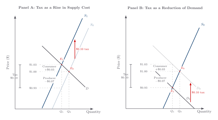
Picture it two ways. Tax the sellers ten cents a gallon and you raise their cost of putting a gallon on the market by ten cents; their marginal-cost curve, and so the supply curve, shifts up by a dime, and the market clears at a higher price. Alternatively, tax the buyers ten cents a gallon. Now at every posted price buyers will pay the seller ten cents less, since the rest goes to the government, so the demand curve sellers see shifts down by a dime. Work either version through and you reach the identical place: the same quantity sold, the same price paid by buyers, the same net price kept by sellers. Whether the law names the buyer or the seller as the taxpayer is a political and emotional detail, not an economic one.

So who ends up paying? In UE’s gasoline example the dime tax raises the price buyers pay by three cents and lowers the price sellers keep by seven cents. The tax splits, with neither side bearing all of it. What sets the split is which side can more easily back away from the deal, the relative responsiveness of demand and supply: the side that can dodge the tax more easily, by cutting back or switching to something else, pushes more of the burden onto the side that is stuck.

That is exactly the error in a case worth remembering. Pittsburgh once put a 20 percent tax on the gross receipts of private parking lots while exempting the city’s own lots. The Supreme Court upheld it and reasoned that, because parking was “in short supply,” operators could pass the whole tax on to drivers, so customers would bear all of it. The economics is wrong. How much of a tax buyers bear has nothing to do with whether something is called a shortage; it depends on the relative elasticities of demand and supply. If drivers can switch to buses, trolleys, or parking elsewhere, the lot operators cannot pass the full tax along and must eat a share of it. A “shortage” does not hand sellers the power to off-load the entire burden.

One more cost of the tax escapes the price split, and we treat it verbally. The tax shrinks the quantity of gasoline produced and consumed. Those gallons no longer made were worth more to buyers than the resources freed up are now worth in whatever else they make. That lost value, the gap between what the foregone gallons were worth and what the displaced resources now produce, is a real cost of the tax, on top of the money the government collects. UE draws it as a measured triangle and calls it a deadweight loss; we keep the plain statement that some genuinely valued output is sacrificed and that loss is nobody’s revenue.

A natural follow-up is to ask who finally gains from all this. We can say with confidence who pays, and that the deadweight loss is a real burden on someone. We cannot say who gains from the tax until we know what the government does with the money it collects. The revenue might fund a bridge, a tax cut elsewhere, or a giveaway to some favored group, and each spends the proceeds on different people. The same caveat is why we cannot pronounce the whole arrangement a net loss to society either: the buyers and the specific-resource owners clearly lose, but whether their loss is outweighed depends entirely on the value of whatever the proceeds buy, which the tax analysis by itself does not tell us. Who pays is an economic question we can answer; who comes out ahead waits on the spending side.

Fixed Land Is the Limiting Case: Its Owner Bears the Whole Tax

The elasticity rule includes a clean extreme. Land in a particular place cannot shrink or move when it is taxed, so its supply is vertical. If a permanent tax is placed on the economic rent of that land, the rent users are willing to pay and the acres in use do not change. The tax is carved out of the owner’s return. This is not a separate exception to tax incidence; it is what the same rule predicts when supply elasticity is zero.

Because a buyer values land by the future income it will yield, a permanent tax lowers the land’s selling price as soon as it is anticipated. Whoever owns the land at that moment bears the loss; a later buyer pays the already-reduced price and earns an ordinary return from there. The acres do not disappear, and the user price does not rise. The burden shows up as a one-time decline in asset value.

Capitalization works upward as well as downward. A new park, safer street, or better local service can raise the stream of advantages attached to nearby land, and buyers bid that gain into land prices and rents. The owner present when the improvement becomes expected captures the windfall; a later buyer pays for it in the purchase price, and a renter or newcomer pays through the higher rent. Only land improved relative to alternatives gains: if every neighborhood receives the same improvement, no one location necessarily acquires a special premium. Calling the benefit “public” does not tell us who finally captures it.

The fixed-land result is the sharp edge of a general rule: a tax settles on whatever cannot get out of its way. Land is the extreme case, since it cannot move or shrink, so its owner absorbs the whole tax through a capitalized fall in value, and it makes no difference whether the law names the renter or the owner as the taxpayer. That is exactly why governments gravitate toward taxing immobile, place-bound bases like land and existing specialized capital, and why proposals to tax land values keep resurfacing, from the nineteenth-century land-tax reformer Henry George and his “single tax” to later arguments for nationalizing land outright. Land cannot flee the tax, so the tax can lean on it.

The converse is the political economy of the whole subject. A base that can move answers a tax increase by leaving, and how much it actually leaves depends on how mobile it is, which varies enormously from one base to the next. The most footloose high earners respond strongly: tracking star scientists through their patents, Moretti and Wilson (2017) found that a state letting these scientists keep 1 percent more of their income drew about 1.8 percent more of them over the long run. The average millionaire, by contrast, stays put. When New Jersey raised its top rate by 2.6 points to 8.97 percent in 2004, the wealthy as a whole barely budged and the tax still raised roughly a billion dollars a year (Young and Varner 2011), with only the mobile slices, retirees and people living on investment income, tending to leave. When a base can exit, the taxing government cannot load the full burden onto it, and the burden slides toward whatever stays put. So jurisdictions compete for the mobile bases, and the taxes that stick are the ones on what cannot leave. Land, which cannot move at all, is the base that stays put no matter what.

That mobility helps explain the politics of a graduated income tax. Several rationales point in the same direction: higher-income taxpayers may be said to have greater ability to pay, to receive more protection for property, or to owe a larger contribution because extra dollars have lower marginal worth to them. There is also a coalition rationale: many voters can impose higher rates on a smaller group. Whatever the justification, rising rates encourage shifts into untaxed nonmarket activity and favored forms of income. Owner-occupied housing makes the point: the homeowner receives an implicit rental service from the house but usually reports no taxable rent, so two households with the same economic income can face different tax bills depending on whether the return arrives in cash or housing services.

Federal revenue sharing is the mirror image of taxpayers escaping a jurisdiction. If a local government bears the political cost of taxing its own mobile residents while neighboring jurisdictions share the benefit of the service, local officials ask a higher level of government to collect the tax and send funds back. The federal grant weakens the taxpayer’s ability to escape by crossing a city or state line. Revenue sharing is therefore not free outside money; it relocates the taxing decision to a jurisdiction from which exit is harder and makes the link between the local service and its local cost less visible.

Before leaving the land case, one more figure closes the loop on who writes the check, this time at the smaller scale of a square foot of rented space. It draws two demand schedules, the renters’ demand and the net-of-tax demand the owner actually faces, and lets you send the tax bill to either side: the same 40 cents comes out of the owner’s rent no matter whose name the law puts on it.

A Tax on a Single Price-Taker Falls Entirely on Him

Change the experiment. Instead of taxing all gasoline, tax exactly one tiny seller, say one peanut farmer out of thousands, a penny a pound on his crop alone. What happens to the market price and quantity? Essentially nothing; his output barely registers in the total, so the market price does not budge. But he cannot raise his own price either, because he is a price-taker, and the market price is set by everyone else. So he sells at the same price as before yet now hands a penny a pound to the government on every pound. The entire burden lands on him, specifically on his specialized land and equipment, whose value drops because they now earn less. It is the mirror image of the broad tax: a tax on everyone splits between buyers and sellers, but a tax on one helpless price-taker is borne wholly by that one seller’s specific resources, since he has no price-setting power to share it.

In the Short Run the Tax Lands on Immobile Resources; in the Long Run on Consumers

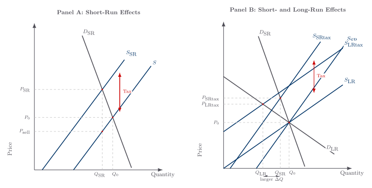
Go back to taxing the whole peanut industry and watch the burden travel over time. In the short run, almost nothing can move. The land is planted, the harvesting equipment is bought and specialized to peanuts, the farmers are committed. Because so little can escape, the immediate burden falls heavily on these immobile resources: their value drops, since they now earn less after tax and cannot quickly shift to other work. But the land and the equipment fall by different amounts, and the reason is worth pausing on. The harvesting, shelling, and roasting equipment is built for peanuts and almost nothing else, so a tax that lowers peanut earnings lowers its value sharply; it has no good second life. The land is not so trapped. It can grow other crops, so it falls in value only to the extent it was worth more for peanuts than for its next-best use. If the land earned about the same growing soybeans, its value barely moves; only the peanut-specific premium is at risk. Redeployable resources lose just their topic-specific edge; fully specialized ones can lose almost everything. Quantity and price each move only a little at first, so producers absorb most of the hit on these fixed, specific assets.

Over the long run, things loosen. Marginal farmers, barely breaking even, give up peanuts and move their resources elsewhere. As output contracts the price rises further, and the survivors’ land and equipment recover much of their lost value, because with fewer producers each remaining one earns more. So the value drop on specific resources is temporary for those who stay. The farmers who exited, though, bear a real and permanent loss: they ate the capitalized fall in their asset values on the way out. And as the price climbs toward covering the tax, consumers increasingly foot the bill at the register. In the long run, with supply more elastic, the tax lands mainly on consumers.

That carries a sharp corollary about latecomers. Suppose years after the tax, demand for peanuts grows, the surviving farms turn profitable, and a fresh investor buys in. How much of the tax does he bear? None of it. The price he pays for land and equipment already has the tax baked in, because their value already reflects the lower after-tax earnings; he earns a normal return on what he paid and carries no part of the burden. The tax was borne once and for all by whoever owned the specific resources when it was imposed. This also disposes of a popular bit of bad public finance, that it is fairer and gentler to “tax businesses, not households.” Taxing the seller and taxing the buyer give the identical result: same quantity, same buyer price, same seller net. Routing a tax through firms rather than people changes who signs the check, not who carries the load.

A new corporate tax follows the same time pattern. At the surprise announcement, the expected after-tax earnings of existing corporations fall and share prices capitalize the loss onto incumbent shareholders. Anyone who buys the shares afterward pays the reduced price and expects an ordinary return; the corporation has not absorbed the burden as if it were a person. Over the longer run, investment can leave the taxed corporate form or move toward less-taxed uses, shifting part of the burden again. The economic question is always which people and resources can adjust, not which legal entity writes the check.

A Resource in Place Earns a Quasi-Rent

The peanut story leans on an idea worth naming. A resource already in place, with its cost sunk, earns what economists call a quasi-rent: a temporary surplus over its bare operating cost.

You can cut that surplus, even cut it hard, without driving the resource out, because its original cost is gone and irrelevant. The only thing that shuts it down is a price so low it fails to cover the cost of operating it, not the cost of having built it. This applies to people too: the gap between what you currently earn and the most you could earn in your next-best job is your quasi-rent, and an employer could trim your pay toward that floor without losing you. The specialized, hard-to-redeploy examples below develop the point.

Cutting Price Below a Rival’s Cost Can Be Efficient, Not Predatory

The quasi-rent idea cracks open a charge you will hear constantly: that a firm cutting its price below a competitor’s cost must be “predatory,” trying to bankrupt rivals unfairly. Often it is nothing of the kind. Imagine an old telephone company, “Old,” that long ago strung copper wire able to carry fifty calls at once. That investment is fully sunk; the wire has no other use. Its costs now look like this.

Old’s existing copper system	Cost per channel per year
Annual depreciation (sunk $1,000,000 / 50 channels, over 20 years)	$1,000
Operating (short-run) cost	$200
Long-run cost per channel	$1,200

Because the $1,000 of capital cost is sunk, Old will keep operating as long as it covers the $200 of operating cost. Anything above $200 a channel is quasi-rent on equipment it has already paid for. Its long-run cost was $1,200, but its short-run floor is only $200.

Now a newcomer, “New,” wants to lay modern fiber. Its costs are different.

New’s proposed fiber system	Cost per channel per year
Capital cost ($1,500,000 / 50 channels, over 50 years)	$600
Operating cost	$75
Long-run cost per channel	$675

At first glance New looks like a winner: $675 long-run cost against Old’s $1,200. But notice what happens if New builds. The market would then hold a hundred channels where there were fifty, and that flood of capacity would drive the price down. Old, with a short-run floor of just $200, can ride the price far below New’s $675 long-run cost and keep operating on its sunk wire. When Old warns New, “build it and the price will fall below your cost,” Old is not making a predatory threat; it is stating a fact about sunk capacity. The wasteful act would be New’s premature investment, sinking $1.5 million into capacity the market does not yet need, not Old’s willingness to keep using equipment it already owns. A price below a newcomer’s long-run cost can be the efficient outcome, not foul play.

Prices Move Before the Event, Because Stored Goods Bridge Present and Future

One last piece of price behavior, because it surprises people and follows from the same logic. Prices often move before the thing everyone worries about actually happens, and they move asymmetrically. Consider coffee. Bad weather damages this year’s crop and the price jumps right away, before any shortfall is felt on the shelf. Why? Because coffee can be stored. Anyone holding beans realizes they will be worth more later, so they hold them off the market today, and today’s price rises immediately to reflect the coming scarcity. Present goods can be carried forward.

Now run it the other way. Word arrives that next year’s harvest will be enormous. Does today’s price fall as sharply? Not really, because future coffee cannot be hauled back into the present. Next year’s bumper crop does not exist yet and no one can sell it today, so today’s price barely moves on the good news. The asymmetry comes straight from storage being a one-way street: you can store present goods forward but cannot pull future goods back. It also explains why “punishing the speculator” for raising prices on bad news is misguided. The price rise is the market doing its job, rationing a now-scarcer good across time.

Creative Destruction Creates More Than It Destroys

Step back from the price-taker firm to the person who shakes the whole market up: the entrepreneur. Real growth comes from someone risking their own wealth on an experiment, a better product or a cheaper way of making an old one. Most such bets fail and the gambler eats the loss; the ones that work displace whatever came before. Joseph Schumpeter called this creative destruction, and the word “destruction” tempts people into thinking it is a wash, that what one firm gains another simply loses.

It is not a wash, and a small example shows why. Suppose Coke spends three cents more a bottle to make a drink consumers value five cents more than Pepsi, and both still sell for a dollar. Buyers switch to Coke. Pepsi loses a dollar of sales on every switcher, so it looks as if the consumer, who gained only five cents of extra worth, imposed a full dollar of cost on Pepsi. That accounting is wrong twice over. First, Pepsi does not lose a dollar; it loses its profit on that bottle, far less than a dollar of revenue. Second, the resources Pepsi no longer uses do not vanish; they move to producing something else worth up to a dollar elsewhere. What looks like a dollar destroyed is really a transfer from Pepsi to consumers plus a reallocation of freed resources. Society is not poorer; it is richer by the improvement. A competitor’s loss to a better product is lost profit, not lost wealth, and the innovator earns a genuine profit precisely because the new value created exceeds the old value displaced.

The same logic explains how a market values resources nobody directly buys. Consumers buy finished goods, yet their willingness to pay for the product flows back, through competition among producers, to set what each contributing resource is worth. The value of the inputs is imputed from the value of the output. No committee assigns it; competition for the resources does, just as competition capitalized a machine’s earnings into its price in Part A.

Firms Rise and Fall as Conditions Change, and That Is the Point

The grandest illustration is the relentless turnover of who is on top. Profits attract entry, losses force change or death, and the firms that read shifting conditions fastest displace the ones that do not. The churn is not a flaw in competition; it is competition working.

Take the A&P grocery chain. For decades it was the largest retailer on earth, and it got there by charging the lowest prices, running on thin margins and enormous volume. Here is a point that confuses many students: cutting its profit margin per item actually raised A&P’s rate of return on investment, because the low prices pulled in so much volume and the goods turned over so fast that the same invested capital earned more overall. Low margin, high turnover, high return. Then the world changed underneath it. Suburbanization, the automobile, and the home refrigerator let a new format, the supermarket, cut costs even further, and shoppers drove to the suburbs to buy in bulk. A&P clung to its central-city stores and was gutted. The firm that won by reading consumers earlier than anyone lost by reading them later.

The same lesson runs backward in time, in the format A&P’s rivals were born into. Sears and Montgomery Ward built their empires on mail order, and geography is why that was the low-cost way to sell. In the early twentieth century, before cars and trucks, most Americans lived scattered across the countryside, and stocking a thousand tiny rural stores with goods was expensive, so rural shoppers paid dearly. Selling by mail from a single huge warehouse and shipping by railroad and the post office skipped all those small local stores and reached a dispersed population at far lower cost, which is exactly why mail order undersold the country store and grew into the largest retailing in the land. Then the population moved. As Americans crowded into cities, the cheapest way to serve them flipped: a chain of urban department stores now beat shipping to scattered homes, and J.C. Penney built one while the mail-order giants hesitated. Sears and Montgomery Ward refused for years to follow their own customers into department stores until red ink finally forced them to move. Eastman Kodak so dominated photographic film that it invented the digital camera in its own labs, then was destroyed by digital photography and went bankrupt, while a rival that diversified survived. The lesson is the same each time: past dominance protects no one. Survival depends on adjusting to what consumers now want, and the firms that fail to adjust are competed out of existence. Consumers, not any particular company, are the lasting beneficiaries.

Losses Are the Market’s Discipline, and No Planner Provides a Substitute

Why does this churn happen under competition but not under central planning? Because of what losses do. In a market, a firm that clings to an obsolete way of doing things runs into red ink, and the red ink eventually forces it to change or shut down. Sears and Montgomery Ward did not abandon mail order because someone persuaded them; they abandoned it because losses made standing still unaffordable. Inertia is human and universal, common under any system. What is special about a market is that it charges for inertia. A system with no losses, where an enterprise cannot fail no matter how badly it serves people, removes that penalty, so inertia persists. The discipline is not in anyone’s good intentions; it is in the unforgiving feedback of profit and loss.

That same discipline runs through one more channel, the only piece of our reputation material I want to pull in here. When a seller competes for repeat business, it is selling its reputation along with its product. Cheat a customer on quality and you may pocket a one-time gain, but you lose that customer and acquire a name that costs you far more future business than the gain was worth, so the prospect of repeat dealing keeps sellers honest with no one policing them. Heinz once sold horseradish in clear glass bottles precisely so buyers could see he was not hiding cheap fillers the way rivals in colored bottles could; a restaurant chain runs surprise inspections of its own suppliers because its name rides on every meal. The market makes honesty pay. A monopoly that cannot be deserted faces no such pressure, one reason we return to the market-versus-government comparison much later.