The Competitive Firm: How a Price-Taker Decides

In T6 we built the cost side of the firm: marginal cost rises as output climbs, and average cost traces a U. What we never did was put a price next to those costs. A cost curve alone cannot tell a firm how much to make, whether to make anything at all, or whether it will survive. For that we need the market price. Part A adds it.

We will study the simplest and most important case: a seller so small relative to its market that it has no power over price. It must take the going price as given and decide only how much to produce. Economists call such a seller a price-taker, and the markets full of them are what we usually mean by “competition.” This is the first of two installments on competitive markets. Part A stays inside a single firm and the industry it belongs to: how a price-taking firm picks its output, how thousands of them together generate a market supply curve, why competition produces the industry’s output as cheaply as possible, and why profits in such a market get driven toward an ordinary return. Part B puts this machinery to work on taxes, timing, and how burdens move as firms and resources adjust.

Figure focus. Required: market-to-firm price and firm cost/output. Others are references unless assigned.

A Price-Taker Faces a Horizontal Demand Curve at the Market Price

Start with a wheat farmer. Wheat sells for $2 a bushel and the whole market trades ten million bushels, of which he grows a thousand. Can he push the price up by withholding his crop? No: a thousand bushels against ten million moves the price by nothing anyone could measure. Can he charge $2.01? Also no. His wheat is identical to everyone else’s, so the instant he asks a penny more, every buyer walks to a rival selling the same grain at $2. And he has no reason to sell for less, since he can already sell every bushel he has at the full $2.

So the farmer can sell as much or as little as he likes, but only at the one price the market hands him. Draw the demand curve facing him alone and it is not the familiar downward slope; it is a flat horizontal line at $2. That flat line is the signature of a price-taker: he takes the market price as fixed and chooses only a quantity along it.

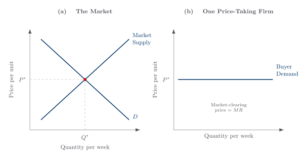
A seller is a price-taker when its own output is too small, and alternatives too close, for its quantity choice to move the market price materially. Homogeneous products help because buyers readily switch; easy entry disciplines profit over time. Neither condition by itself guarantees a horizontal firm demand curve: a handful of large sellers may affect price even if entry is possible, while many differentiated sellers may retain some pricing discretion. Price-taking is a benchmark about the firm’s residual influence, not a literal head-count test.

Set aside, for now, a different kind of seller: one that faces a downward-sloping demand for its own product, so that to sell more it must cut its price. Such a seller does not take a price; it searches for one. We study those price-searchers in a later topic.

For a Price-Taker, Marginal Revenue Is Just the Market Price

Because our farmer can sell any quantity at the same $2, the revenue from one more bushel is easy to find: sell one more and revenue rises by exactly $2, with no hidden cost from a lower price on everything else, since selling more does not move the price. The extra revenue from one more unit is what we call marginal revenue. For a price-taker, marginal revenue equals the price.

That is precisely what fails for a price-searcher, who must cut its price to move extra units and so earns less than the price on each new sale, since the cut bites into the units it was already selling. For that seller marginal revenue falls below price. Competition behaves so cleanly because, for a price-taker, marginal revenue and price are the same number.

The Firm’s Supply Curve Is Its Rising Marginal Cost

Now we can answer the first decision: at a given price, how much should the firm make? Run the marginal logic from T6: as long as one more unit brings in more than it costs, make it. The price-taker’s marginal revenue is the price, so the rule becomes keep producing until marginal cost rises to meet the price. Produce less and you leave units on the table that would have earned more than they cost; produce more and each extra unit costs more than it fetches.

Put numbers on it with a single producer’s cost schedule, the same figures from T6, now with a market price attached.

Daily rate of production	Marginal cost	Average variable cost	Average total cost
0	—	—	—
1	9	9.0	19.0
2	8	8.5	13.5
3	6	7.7	11.0
4	5	7.0	9.5
5	7	7.0	9.0
6	13	8.0	9.7
7	22	10.0	11.4
8	30	12.5	13.8
9	40	15.5	16.7
10	51	19.1	20.1
11	65	23.3	24.2
12	80	28.0	28.8

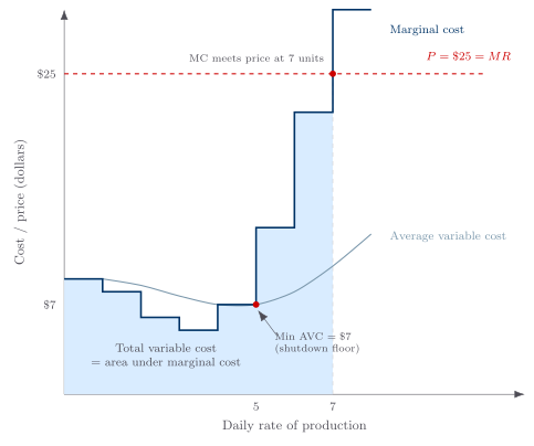
Suppose the market price is $25. Where does marginal cost meet it? At seven units. The seventh unit costs $22 to make and sells for $25, so it is worth producing. The eighth would cost $30 and still fetch only $25, so making it would shrink profit by $5. Seven units is the profit-maximizing rate, found without ever consulting average cost; the marginal comparison alone pins down the rate.

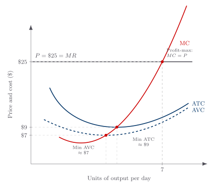
Read the table the other way and the firm’s supply curve falls right out of it. At $25 the firm offers seven units; at a higher price it would push to eight, nine, ten, climbing its marginal-cost schedule. What the firm is willing to supply at each price is read straight off its rising marginal cost. That is the deep result: above a certain floor, the firm’s marginal-cost curve is its supply curve. We pin down that floor next.

Shut Down or Keep Going Depends on Whether Price Covers the Right Cost

Finding the best rate is only half the decision; the other half is whether to produce at all, and a famous slogan does the work: marginal cost guides how much to produce, while average cost tells you whether to produce. Confusing the two is one of the most common mistakes in economics. Marginal cost versus price sets the rate, as we just saw; whether running at all earns or loses money compares price with average cost. But there are two average costs, one for each time horizon, each with its own threshold.

In the short run, the firm has already sunk money into its building and machinery. That money is gone whether the firm produces or not, so it should not enter a decision about today’s output; what matters is only the cost that changes with production, the average variable cost. As long as price covers average variable cost, every unit pays its own running expenses and chips in something toward the sunk investment, so the firm keeps going. In our table average variable cost bottoms out at $7: above $7 the firm keeps producing with the equipment it has, below $7 it shuts down.

The long run is a different decision program, not the same one stretched out. Once the equipment finally wears out, buying new machinery is a fresh, avoidable cost rather than a sunk one. Now the relevant figure is average total cost, which includes the cost of capacity. It bottoms out at $9 in our table, so the firm reinvests and stays in business only if the expected price covers at least $9; below $9 it runs the equipment it has until it dies, then exits.

There is the floor we promised. The firm’s marginal-cost curve serves as its supply curve only above the lowest average variable cost, $7; below that it produces nothing. And the lowest average total cost, $9, is the price below which it will not stay in the industry permanently. Same firm, two break-even prices, because the short run and the long run are two different production plans, each carrying its own cost.

Add Up Every Firm’s Supply and You Get the Market Supply Curve

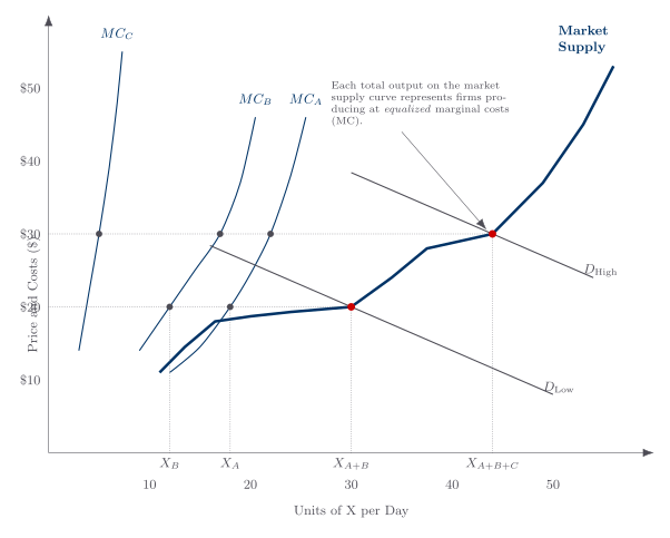
One firm’s supply curve is its marginal cost above the shutdown point, and a market is full of such firms. To get the supply curve for the whole market, ask at each possible price how much every firm would produce and add those quantities together. That horizontal sum, across all firms, is the market supply curve.

For a fixed set of firms in the short run, it slopes upward because each firm’s marginal cost rises with output and some previously idle capacity begins operating. Entry and exit are separate long-run margins. A higher expected price can draw in firms, but the long-run industry’s slope also depends on whether entry bids up input prices, brings costs down, or leaves them unchanged. The horizontal sum is therefore the short-run construction; long-run supply incorporates how the population and costs of firms change.

Competition Pushes Every Firm’s Marginal Cost Toward the Same Number

Here is the benchmark result. Every price-taker expands until its own marginal cost equals the one market price. If firms make the same product, face prices reflecting opportunity cost, and create no omitted external effects, their marginal costs converge. That allocation minimizes the measured resource cost of producing the given industry output.

Suppose one more identical unit costs $5 in one firm but $6 in another. Shifting production toward the first can deliver the same output for less until marginal costs equalize. Market prices can induce that reshuffling without a planner calculating each move. The conclusion is deliberately narrow: it is cost minimization for a specified output under the benchmark, not proof that the distribution is fair, every cost is priced, or the output itself is normatively best.

Survival, Not Conscious Optimizing, Is What Competition Selects For

I have been talking as though each owner equates marginal cost to price on a spreadsheet. Real managers rarely know their costs that precisely; they have hunches about pushing output higher or pulling it back, but the exact marginal cost of the next unit is usually a fog. Does the analysis collapse?

The market does not require anyone to calculate the optimum. Losses, takeover, entry, and exit pressure firms that stray far from sustainable choices, while firms landing nearer the profitable range are more likely to survive and grow. This is a selection tendency, not a guarantee: luck, finance, regulation, market power, managerial goals, and unpriced effects can preserve departures or eliminate capable firms. Marginal conditions describe a benchmark toward which competition pushes, not arithmetic every manager performs or an assurance that every survivor is best.

Profits Turn Into Costs as Rivals Bid for Whatever Earns Them

Now to the engine that drives competitive profits toward an ordinary return. The usual story says competition “competes profits away” but rarely explains the mechanism, which is that profits get converted into costs.

Follow a single machine. An investor pays $10,000 for it, expecting 5,000 units of output at $1 per unit in other inputs, and hopes to sell the product for $3, just covering the machine. Then luck breaks his way and the product sells for $4. Each unit now clears $3 over the other-input cost, so over its life the machine throws off $15,000 instead of the $10,000 it cost. Once rivals expect that earning stream to persist, they bid for the machine. The profit has been capitalized into the machine’s price. In this simplified table with no discounting or risk, its value rises to $15,000; a later buyer earns an ordinary return from that price. In practice the bid reflects expected future net earnings, timing, risk, taxes, bargaining, and alternatives, which T11 will make explicit.

The table tracks the machine as the product price moves.

Case	Product price	Net unit earnings (after $1 other inputs)	Machine’s value in use (= net unit × 5,000)	Cost of using the machine, per unit	Outcome
A	$4.00	$3.00	$15,000	$3.00	Invest; profit of $5,000 over the $10,000 paid
B	$3.50	$2.50	$12,500	$2.50	Produce; profit of $2,500
C	$2.00	$1.00	$5,000	$1.00	Keep producing; profit of $0
D	below $1	near zero	about zero	—	Terminate; the machine is worth scrapping

Two lessons live in that table. First, the cost of using the machine is not the $2 per unit computed from its $10,000 purchase price; it is whatever the machine is currently worth, spread over its output. When the product sells for $4, the true cost of using the machine is $3 a unit, because that is what you sacrifice by using it rather than selling it. The historical price paid is irrelevant; only current value counts. That kills a stubborn fallacy, that new firms can undercut old ones because the old are “burdened” with obsolete equipment. They are not: old equipment is continuously revalued to whatever level lets it keep competing, and at that lower value it competes on equal footing with anything new. What a firm once paid for its capital is dead history.

Be precise about sources. Entrepreneurial profit is an unanticipated increase in wealth when realized value exceeds the opportunity cost of the resources used. A scarcity rent can arise from a scarce location, talent, patent, network, or legal restriction. A policy-created restriction may transfer value to its holder without increasing total output, while an innovation can create value and still confer temporary market power. Accounting profit alone does not reveal which story applies; entry conditions, rights, external effects, and counterfactual output do.

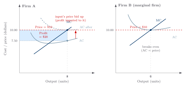
When rivals bid up the price of a profit-earning asset, what they pay for is its stream of future earnings squeezed into a single price today. Collapsing a future flow into a present price is capitalization, and we will make its arithmetic explicit when we reach present value and capital later. For now the verbal version is enough: tomorrow’s profit gets baked into today’s asset price, leaving the new owner only a normal return.

Is Producing Where Price Equals Marginal Cost Socially Desirable?

Competition pushes each firm to produce where price equals marginal cost. Under a specific benchmark, that is productively and allocatively efficient; it is not a complete welfare verdict.

If willingness to pay measures marginal personal worth, marginal cost includes every opportunity cost, exchange is voluntary and informed, and no effect falls on outsiders, the last unit is worth as much to the person who gets it as the resources sacrificed. Lower output forgoes units valued above cost; higher output uses resources worth more elsewhere. Distribution, rights, information, public goods, and external effects require additional analysis. The benchmark establishes exhausted gains under its assumptions, not that every competitive outcome is socially best.

For Further Reading

Want to explore the source material? This lecture draws on the following chapters from two books by Armen A. Alchian and William R. Allen:

• Universal Economics (Liberty Fund, 2018): Ch. 16, “Market Supply and Price with Price-Takers”.
• Exchange and Production, 3rd ed. (Wadsworth, 1983): Ch. 10, “Price Takers’ Supply and Price Response to Consumer Demand”.

• Price-taking now rests on negligible residual price influence, not homogeneity/entry as a sufficient two-condition theorem; short-run summation is separated from entry.
• Equal-MC and P=MC conclusions name their opportunity-cost, information, and external-effect assumptions; selection is pressure, not proof of survivor optimality.
• Capitalization retains the machine table while adding expectations, timing, and risk; entrepreneurial profit, scarcity rent, and policy-created transfer are distinguished.
• Three objectives, ten Core/fourteen coverage anchors, four figures, and routing remain. —>