Marginal Analysis, Production, and Costs

Back when we studied trade, I left you with a promise and a puzzle. The promise was a second, deeper source of gains from exchange that we had not yet touched. We had explained how trading makes everyone richer because people value the same goods differently, and I said something else was going on too: people also differ in what it costs them to make things. The puzzle was a claim that sounds impossible: you can be worse at producing everything than the person next to you and still have something worth selling to them.

We make good on both across this two-part topic. Part A first builds the total/marginal/average and equimarginal tools, then asks a question that seems too simple to bother with: what does it actually cost to produce something? The honest answer is surprising, and once we have it the rest follows, including the resolution of that puzzle, why a less talented person can still be the cheaper producer of something, and a handful of cost ideas that will do real work throughout the course. Part B puts this machinery to use on specialization and exchange.

Totals, Marginals, and Averages Answer Different Questions

Production gives us the right home for a general toolkit that we will reuse for cost, output, revenue, and hiring. For any quantity, the total is the running sum, the marginal is the change in that total caused by one more unit, and the average is the total divided by the number of units. They travel together, but they answer different questions.

Suppose a worker scores 80 on a first quality check, 86 on a second, and 89 on a third. The three marginal observations are 80, 86, and 89; the totals are 80, 166, and 255; and the averages are 80, 83, and 85. The new observation pulls the average toward itself. A marginal above the current average raises the average; a marginal below it lowers the average; and a marginal equal to it leaves the average unchanged. This marginal-average rule is arithmetic, not a special feature of test scores. It governs average product and average cost too.

The decision-relevant number is usually marginal. A store’s sales rise from $1,000 with one clerk to $1,800 with two. The second clerk’s marginal contribution is $800, the change in the store’s total, even if that clerk personally rings up a different amount. The same reasoning applies to a factory deciding whether to add a shift: compare what the next shift adds with what it costs. An average summarizes all units already chosen; the marginal tells you what changes if you choose one more.

Revenue uses the same arithmetic. Suppose a chair seller can sell one chair for $110 but must cut the price to $100 to sell two. Total revenue rises from $110 to $200, so the second chair’s marginal revenue is $90, not its $100 selling price: the lower price also costs the seller $10 on the first chair. Average revenue is $100 per chair. The details of how a price-setting seller uses marginal revenue belong to market power; the general lesson here is that a marginal is always the change in the total, not merely the amount attached to the newest unit.

Efficient Allocation Equalizes Marginal Returns Across Uses

The toolkit becomes most useful when a producer has a fixed resource and several places to put it. Suppose ten machine-hours can be split between production lines A and B. Line A’s first hours are very productive but its marginal return falls quickly; line B begins lower but declines slowly. Sending every hour to whichever line has the larger total return is the wrong comparison. The producer should assign each next hour to the line offering the largest remaining marginal return.

In the worked schedule, the best split assigns four hours to A and six to B. That combination produces a total return of 150.5, more than putting all ten into A (110) or all ten into B (127.5). At the best integer split, the last hours assigned to the two lines have nearly equal returns. Moving an hour from one line to the other would give up more at the source than it adds at the destination.

This principle is not an extra rule laid on top of production. It is the logic connecting a production schedule to a decision. The same scarce hour cannot be in both factories, so its opportunity cost in one use is the marginal return forgone in the other. Efficient allocation keeps moving units until no such move can raise the total.

The mirror rule for costs has a policy history worth knowing. During the 1970s energy crisis, federal rules allocated crude oil across refiners by administrative formula rather than by price. The Emergency Petroleum Allocation Act, signed in November 1973, led to a Crude Oil Entitlements Program in November 1974 that equalized refiners’ crude costs through monetary transfers between them. The Energy Policy and Conservation Act of 1975 then added a small-refiner bias, granting extra entitlements to refineries of 175,000 barrels a day or less, with the largest bonus reserved for those processing 10,000 barrels a day or less. Because the subsidy flowed toward the smallest, highest-cost “tea kettle” plants, it pulled production toward refiners a common price would have shut out. Federal auditors found that 64 refineries began operating between 1974 and 1980, all but two below 50,000 barrels a day, and many closed once price decontrol in January 1981 ended the subsidy. Equalizing marginal cost across producers is exactly what a common price does on its own; an administrative rule that props up high-cost capacity does the opposite, and makes the same output at more than its least possible total cost.

The Cost of Producing Something Is the Best Thing You Give Up to Make It

Ask a businessperson what a product costs and you will hear a number: so much for materials, labor, and machines. That accounting figure has its uses, but it is not what an economist means by cost. The cost of making something is the most valuable other thing those same resources could have produced instead. This is the same idea we met on the first day, opportunity cost, now pointed at production rather than personal choices. Every cost is a sacrificed opportunity. The dollars on the invoice matter only because they measure what those resources would have fetched in their best other use.

This is why we do not measure costs in labor hours, tempting as that is. An hour is not an hour. A surgeon’s hour and a shelf-stocker’s hour command wildly different pay because they can produce wildly different value elsewhere. An hour is worth its best alternative use, not the reading on the clock, so “it took 200 hours to make” tells you almost nothing about cost until you know what those hours could otherwise have done.

One more confusion controls everything that follows. Being more productive at making something is not the same as being a lower-cost producer of it. A baker who churns out twice as many loaves per day as her neighbor is more productive, but that does not yet tell us her loaves are cheaper, because the cost of a loaf is the soup or pies she gives up to bake it, and we have not asked what she gives up. Productive ability is about how much you can make; cost is about what you forgo to make it.

No One Can Be the Low-Cost Producer of Everything

Here is the claim that pays off the puzzle from our trade lesson. Take Bill and Susan, who can each spend a day making jam or cake. Susan is the more gifted producer: in a day she can make more jam than Bill and more cake than Bill. She has what we call an absolute advantage in both goods, meaning she is simply better at making each of them.

You would think the better producer must be the cheaper producer of everything. She is not, and seeing why is the heart of this topic. The cost of a cake is not measured in talent. It is measured in the jam given up to make it. Watch what happens when we line up their abilities and then ask what each one gives up.

Producer	Can make in a day	Cost of one cake (in jam given up)	Cost of one jam (in cake given up)
Bill	5 jams or 10 cakes	0.50 jam	2.0 cakes
Susan	10 jams or 15 cakes	0.67 jam	1.5 cakes

Table 1 (after UE Table 14.1). Susan can out-produce Bill at both goods, yet Bill is the lower-cost maker of cakes: each cake costs him only half a jam, while it costs Susan two-thirds of a jam. Absolute talent and low cost are different things.

Bill, to make one cake, gives up half a jam, because in the time it takes him to make ten cakes he could have made five jams. Susan, to make one cake, gives up two-thirds of a jam. So even though Susan is the more talented cake-maker in absolute terms, Bill is the cheaper cake-maker, because he sacrifices less to produce one. Susan, in turn, is the cheaper jam-maker.

This is not a fluke of these numbers but a law of arithmetic. No matter what abilities you write into that table, one person cannot have lower costs in both goods, because cost in one good is just the flip side of cost in the other: if Susan gives up little jam per cake, she must give up a lot of cake per jam. The conclusion is completely general: no one can be the lowest-cost producer of everything, which means everyone is the lowest-cost producer of something. We call the thing you give up the least to make your comparative advantage. There is the answer to the puzzle. You can be worse at making every single good, like Bill, and still be the cheaper producer of one of them, and that is exactly what gives you something worth selling. Part B cashes this in: that gap in costs is the whole engine of specialization and trade.

One tempting mistake to nail: “a lower-cost producer can produce more than a higher-cost producer” sounds reasonable and is false. Cost tells you what someone gives up per unit; it says nothing about how many units they can crank out. Bill is the low-cost cake-maker yet can make fewer cakes per day than Susan. Low cost and high volume are separate questions.

Marginal Cost Rises as You Produce Faster

The jam-and-cake story kept costs flat: every cake cost Bill the same half-jam. Real production is rarely that tidy. To see how costs actually behave, meet Adam, who spends his days making cakes and could instead be making a whole basket of other goods. We will bundle everything else he could produce and call its dollar value Y, so we never have to track which particular other goods he forgoes. The cost of a cake, then, is the value of Y he gives up to bake it.

Two cost ideas need separating. The average cost of cakes is total cost divided by the number of cakes. The marginal cost is the addition to total cost from making one more cake, the cost of the next one specifically. They answer different questions, and confusing them causes no end of trouble.

Cakes per day	Total cost (in Y)	Marginal cost (next cake, in Y)	Average cost (per cake, in Y)	Other goods Y still producible	Marginal worth of the cake (in Y)
0	—	—	—	13.50	—
1	0.90	0.90	0.90	12.60	1.15
2	1.90	1.00	0.95	11.60	1.05
3	3.00	1.10	1.00	10.50	0.95
4	4.20	1.20	1.05	9.30	0.85
5	5.50	1.30	1.10	8.00	0.75
6	6.90	1.40	1.15	6.60	0.65
7	8.40	1.50	1.20	5.10	0.55
8	10.00	1.60	1.25	3.50	0.45
9	11.70	1.70	1.30	1.80	0.35
10	13.50	1.80	1.35	0.00	0.25

Table 2 (after UE Table 14.2). Adam’s cost of cakes. Read down the marginal-cost column: each successive cake costs more Y than the one before. The marginal worths in the last column fall as he eats more cake. Adam stops where they cross.

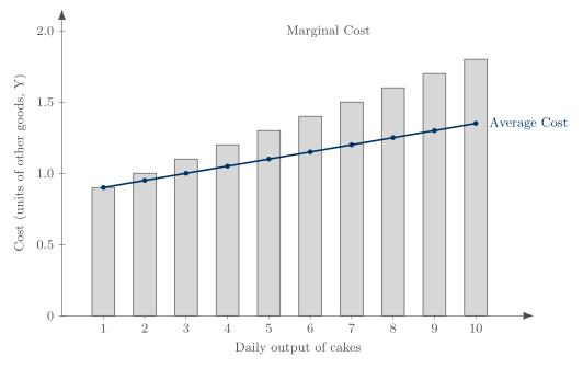
Look at the marginal-cost column. The first cake costs Adam 0.90 of Y; the second costs 1.00; the sixth costs 1.40. Marginal cost rises as he produces faster. Two relationships are baked into this table. First, the marginal costs add up to the total: the total cost of six cakes (6.90Y) is exactly the sum of the marginal cost of each of the first six. Second, marginal cost pulls average cost along with it. When the next unit costs more than the current average, it drags the average up; when it costs less, it pulls the average down; when it equals the average, the average holds still.

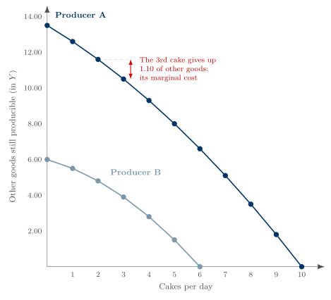
A running back illustration makes that stick. He averages five yards a carry coming into the game, breaks off a six-yard run, and his average ticks up, though not all the way to six. Then he gets stuffed for two yards and his average slips back down. The most recent carry, the marginal one, tugs the average in its own direction. Cost works the same way, which is why a rising marginal cost eventually drags average cost up behind it.

Diminishing Marginal Returns Is Why Faster Costs More

Why does marginal cost rise as you produce faster? Part of it is that to go faster you press the second-best equipment into service. But the deep reason has a name and no exceptions: the law of diminishing marginal returns. As you add more of one input to a fixed amount of the others, the extra output from each additional unit of that input must eventually fall.

Units of the variable input	Total product	Marginal product (next unit)	Average product (per unit)
0	0	—	—
1	6	6	6.0
2	16	10	8.0
3	24	8	8.0
4	30	6	7.5
5	34	4	6.8
6	36	2	6.0
7	36	0	5.1
8	32	−4	4.0
9	27	−5	3.0
10	21	−6	2.1

Table 3 (after UE Table 14.3). Adding more of one input to fixed others. The marginal product climbs at first, peaks at the second unit, then falls, and eventually goes negative so that total product itself drops. Notice the same marginal-pulls-average rule: once marginal product sinks below the average, it drags the average down.

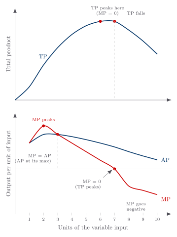
The reductio is unforgettable. If returns did not diminish, you could grow all the world’s wheat in a single flowerpot, just cramming more seeds and fertilizer into that one fixed pot of soil to harvest as much grain as you please. Obviously you cannot, because the fixed input, the pot, gets crowded: each new seed has less soil, water, and light than the one before. The same crowding is why a kitchen that turns out cakes faster eventually strains its fixed oven and floor space, so each extra cake costs more than the last. Marginal cost rises because marginal product falls. This is a fact of physical production, not a story about prices going up.

That distinction matters. Suppose you could exactly clone all of Adam’s inputs, doubling the kitchen, oven, and labor at once. That move need not raise the cost of a cake, because nothing is being crowded; you have simply built a second identical operation. Diminishing returns bites only when you add more of one thing to a fixed amount of the rest. It does not come from input prices rising.

Rate and Volume Are Two Different Cost Questions

A second distinction hides in the word “more,” and it trips people constantly. Producing “more” can mean two unrelated things: a faster rate (more cakes per day) or a larger total volume (more cakes over the life of the operation). They push cost in opposite directions.

The travel analogy fixes it. The cost of a trip depends on your speed and on the distance, and you would never confuse the two. Driving faster burns more gas per mile, just as producing at a faster rate raises marginal cost, for the diminishing-returns reason we just saw. But covering a greater total distance, or producing a greater total volume, is different: a larger volume invites cheaper methods. When Ford builds a few cars, hand tools make sense; when it commits to millions, mass-production machinery that would be absurd for a handful becomes the cheapest way, and the cost per car falls. A hand hammer beats a power hammer for a few nails and loses badly for a few thousand. So faster generally means costlier per unit, while bigger total volume means cheaper per unit. When someone says production went “up,” ask: faster, or more in total?

Volume can lower cost even when the equipment stays the same, because people learn by doing. Repetition reveals better component designs, sequences, and production methods, so the marginal cost of later units falls as cumulative output grows. This learning curve helps explain the familiar path of a new product: early versions sell at high prices to buyers with high marginal worths; experience, larger volume, and entry then lower costs and prices, bringing the product within reach of more buyers. A falling real price can therefore be evidence of learning and competition, not proof that the early price was exploitative or that the later one is predatory.

Joint production adds one more cost lesson. A steer produces beef and hide together; an aircraft carries passengers and freight with many of the same inputs. There is no uniquely correct way to divide the common cost between the joint products, and managers do not need one. The actionable question is how much total cost changes when one more passenger, pound of freight, or increment of feed is added. Allocate shared overhead however an accountant must, but base the production decision on the change in total cost caused by the choice.

A Producer Stops Where the Next Unit’s Worth Falls to Its Cost

Here is the production-side version of a rule you already know from demand. How many cakes should Adam make if he is on his own, both baking and eating them?

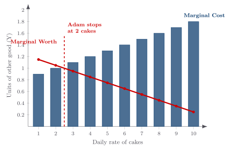
Look at the last column of Table 2, the marginal worth of each cake to Adam, the most Y he would give up to have it. As we saw on the first day, the more cake he already has, the less he will give up for one more, so those worths fall: 1.15, 1.05, 0.95. His marginal costs, meanwhile, rise: 0.90, 1.00, 1.10. Adam keeps baking while the next cake is worth more to him than it costs. The first is worth 1.15 and costs 0.90; the second is worth 1.05 and costs 1.00; the third would cost 1.10 but is worth only 0.95, so he stops at two cakes a day.

That is the stopping rule, and it is the mirror image of demand: a producer makes a good up to the point where its marginal worth, or its price, has fallen to its marginal cost, and not one unit further. This rising marginal-cost relationship is the single most useful thing you will carry out of this topic, because it is what a firm reads off to decide how much to produce in competitive markets. It reads its decision straight off the marginal-cost curve built here.

High Wages Are Not the Same as High Costs

Before we leave the cost machinery, let me defuse a fallacy you will hear your whole life. “We can’t compete with cheap foreign labor; their workers earn a fraction of ours, so their goods must be cheaper.” The mistake is treating the wage, the price of an hour of labor, as if it were the labor cost per unit of output. The gap between them is productivity.

	Wage per hour	Units of output per hour	Labor cost per unit
US worker	$20	10	$2.00
Foreign worker	$10	3	$3.33

Table 4 (after UE Table 14.4). The higher-wage worker is the lower-cost worker. Labor cost per unit is the wage divided by output per hour: the US worker earns twice as much per hour but produces more than three times as much, so each unit carries less labor cost.

The arithmetic is just wage divided by output. The American earns twice the wage but produces more than three times the output per hour, so the labor cost baked into each unit is lower, two dollars against three and a third. A worker paid more per hour can be the cheaper input per unit, as long as she makes enough more per hour to cover the higher pay. High wages usually signal high productivity, and high productivity is exactly what makes a unit cheap to produce. So when someone points at a low foreign wage and predicts cheap imports, ask the question the wage alone cannot answer: how much does that worker produce per hour?

Productivity Depends on Everything Around the Worker, Not the Worker Alone

That last point opens a bigger one. We have been treating cost and productivity as properties of a person. They are not, quite. How much a worker produces depends heavily on what surrounds her: the tools, the management, the co-workers, the whole setting. This cuts against our instinct to read high output as personal merit.

Give a worker more and better capital and her output per hour climbs. A hammer in a poor country actually drives more nails per year than a hammer in a rich one, which sounds backward until you see why: capital is scarce there, so each tool is shared among more workers and used more intensely, while in a rich country tools are plentiful and each sits idle more of the time. The scarce resource gets economized hardest where it is scarcest. Management matters too: Japanese-run textile mills in 1930s China produced cloth at a lower labor cost per unit than Chinese-run mills using the very same machinery, because the work was organized better. Even an athlete’s measured output reflects his circumstances; a slugger hits more home runs partly because of who bats behind him, since pitchers cannot afford to walk him when a dangerous hitter waits on deck. Be careful equating someone’s output with his merit. Output is a joint product of the worker and everything working alongside him.

Capital and Labor Substitute, and “Efficiency” Has No Meaning Until You Name the Goal

Because tools and workers together make output, a firm can often produce the same thing with more machines and fewer people, or the reverse. Capital and labor substitute for each other, and which mix is cheapest depends on which input is scarcer and costlier. Make labor artificially expensive, say by forcing bus drivers’ pay well above the market rate, and firms economize on the now-pricey labor: they run longer buses with one driver carrying twice the passengers and let the gaps between buses stretch, so riders wait longer. Poor countries, where capital is scarce, lean on abundant labor; rich countries, where labor is dear, lean on abundant capital. Neither mix is “right” in the abstract. Each economizes on whatever is scarcest locally.

That brings us to a word people throw around as if it were obvious: efficiency. Efficient at what? American agriculture once looked wildly inefficient measured by output per acre and was the envy of the world measured by output per worker, because land was plentiful and farm labor scarce, so the sensible thing was to economize on labor, not land. Whether the hammer driving more nails in a poor country is “more efficient” depends entirely on which scarce resource you are trying to stretch. There is no efficiency in the abstract, only efficiency relative to a goal, the same lesson we drew on the first day when we called efficiency a no-waste test that cannot, by itself, tell you which point to aim for. Name the goal first; only then does “efficient” mean anything.

Once a goal is named, we can say precisely what efficient production means, and there are two ways to say the same thing. One: production is efficient when the output of one good is as large as it can be for whatever amounts of the other goods you have chosen to make. Two: production is efficient when you cannot make more of one good without making less of another. The two phrasings are equivalent. Each says that nothing is being wasted, that you have squeezed everything possible out of the resources, so the only way to get more of one thing is to give up some of another. Notice that this definition does not assume anyone has perfect knowledge. Efficient production uses the knowledge that actually exists and lets it be tested against results; knowledge is itself a costly resource, so being ignorant of something is not always wasteful or irrational, since gathering the information would have had its own cost.