Demand and Marginal Personal Worth

The opening topic ended with the idea that begins our work on demand: the more of something you already have, the less you will give up to get one more unit of it. Underneath it is a plain fact: people value things differently, and the value they place on one more unit changes as they get more of it. Here we put that fact under a microscope and describe how the amount people are willing to buy responds to price. Out of that description comes the most reliable principle in all of economics and a way of cutting through one of the slipperiest words in public debate: “need.”

Keep one puzzle in mind. Almost everyone agrees that people “need” food, housing, medicine, and clean water. We call some of those needs urgent, others basic or vital, as if the label by itself established how much must be supplied, cost aside. Yet the moment you ask “how much, and at what price?” trade-offs reappear. By the end of this post you should see why a need label does not determine a fixed quantity demanded, and why saying so does not deny biological requirements or the urgency of human wants.

Figure focus. Required: slide versus shift; marginal worth and surplus. Others are references unless assigned.

At a Higher Price People Buy Less, at a Lower Price They Buy More

Start with what we will call the first law of demand:

That is it. It is the most dependable regularity economists have, and almost nothing in the course will contradict it.

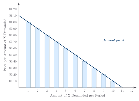
The word demand needs care, because we use it precisely and the world uses it loosely. By a person’s demand for a good I do not mean the single amount they happen to buy at today’s price. I mean the whole schedule: how much they would buy at each of the prices they might face. Think of it as a snapshot taken at one moment, not a record of purchases made one after another as price drifts over time. Here is such a schedule for one person’s weekly purchases of milk.

Price of a quart	Quarts demanded per week
$1.00	1
$0.90	2
$0.80	3
$0.70	4
$0.60	5
$0.50	6
$0.40	7
$0.30	8
$0.20	9
$0.10	10

Read the schedule as that snapshot, not as a purchase diary, and a few common errors disappear. Plotted on a graph, with price up the vertical axis and quantity along the horizontal, it traces a curve that slopes downward to the right. The exact shape, whether straight or bowed or stepped, does not matter; holding the other conditions that define this schedule fixed, its tilt is negative.

Notice too that “quantity” is richer than a simple count. Suppose someone protests that cheaper vacations should make them take more, yet they still take just one a year, so the law must be wrong. It is not: a larger quantity of vacation can mean a longer, fancier, or more frequent one, not just a higher number on the calendar, and you respond to a lower price along whatever margin is open to you.

The law does not claim that buyers carry a numerical schedule in their heads or calculate at the register. It describes behavior when options change, not a thought process. Because purchases can be discrete, a small price change may leave quantity unchanged; the claim is that some sufficiently higher price reduces it, holding the demand schedule fixed. Buying more at a higher price would require some other condition to change or the unusual wealth effect examined next.

A Change in Price Slides Along the Curve; Other Conditions Can Shift It

This is the single most important distinction in the topic, and the one students most often botch on exams. Two completely different things can change how much of a good gets bought, and economics gives them different names.

If the good’s own price changes, you move along a fixed demand curve to a new quantity. We call that a change in the quantity demanded. The curve has not moved; you have slid to a different point on it. A drop in the milk price from $0.60 to $0.50 takes our buyer from five quarts to six, both points on the same schedule above.

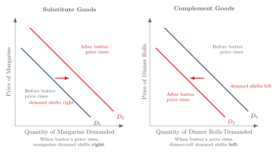
If some other relevant condition changes how much the buyer wants at the possible prices, the curve shifts. We call that a change in demand itself. An increase shifts it rightward; a decrease shifts it leftward. For one buyer, income, related-good prices, tastes, and expectations can matter. A market demand curve sums all buyers’ quantities at each price, so the number of buyers can shift it while individual schedules stay fixed. A non-own-price change shifts a curve only if it changes the choices represented there.

Run a quick test: what raises the demand for wigs? A raise in your salary, a rise in the price of hats, a new swimming pool in town, costlier hair care, a divorce, more people around you wearing wigs, a lower price for wigs themselves. Every item on that list except the last shifts the demand curve, because each is something other than the wig’s own price. The lower wig price is the odd one out: a movement along the curve, a change in quantity demanded, not a change in demand. Ask first whether the good’s own price changed or something else did; that answer tells you whether to slide or to shift.

The related-goods case deserves a name of its own. Some goods are substitutes: a rise in the price of butter raises the demand for margarine, because people switch toward the cheaper alternative, shifting margarine’s whole curve to the right. Other goods are complements, used together: a rise in the price of butter lowers the demand for dinner rolls, shifting that curve to the left. We tell substitutes from complements by which way one good’s price shifts the other’s demand.

The Height of the Demand Curve Is What One More Unit Is Worth to You

Why does the demand curve slope downward in the first place? The answer needs a name for what one more unit is worth to you.

Your marginal personal worth of a good is the most you would pay for one more unit of it. On the demand schedule, it is exactly the height of the curve at that quantity.

Look again at the milk buyer, now with the worth of each successive quart spelled out.

Price	Quantity	Marginal personal worth	Total personal worth
$1.00	1	$1.00	$1.00
$0.90	2	$0.90	$1.90
$0.80	3	$0.80	$2.70
$0.70	4	$0.70	$3.40
$0.60	5	$0.60	$4.00
$0.50	6	$0.50	$4.50
$0.40	7	$0.40	$4.90
$0.30	8	$0.30	$5.20
$0.20	9	$0.20	$5.40
$0.10	10	$0.10	$5.50

The buyer purchases a second quart only when the price falls to $0.90, which tells us the second quart’s marginal worth is $0.90. The total personal worth of two quarts is the sum of the first and second, $1.90, found by adding down the marginal column. That total is not the price times the quantity: two quarts bought at $0.90 each cost $1.80, but they are worth $1.90.

That distinction clears up a question that trips people. Suppose someone buys five units at $0.60 and six units at $0.50, spending exactly $3.00 in both cases. Does that mean the sixth unit is worth nothing, since total spending did not change? No: the sixth unit is worth its marginal worth, $0.50, the price at which the buyer was just willing to take it. The unchanged total is a quirk of the arithmetic, not a statement about the sixth unit’s value. Likewise, if a buyer would pay up to $0.90 for a second unit, it does not follow that each of the two units is worth $0.90; only the second, the marginal one, carries that worth, and the first was worth more. By “value” I mean something concrete: the amount of other goods, measured in dollars for convenience, that a person will actually give up to get the good. Not what they say but what they will give up.

Now the reason for the downward slope. The more of a good you already have, the less you will give up for one more unit. Economists call this diminishing marginal personal worth, readable straight down the marginal column above: each additional quart is worth less than the one before. Because marginal worth falls as quantity rises, the curve that plots worth against quantity slopes down; that is the engine under the first law. Marginal worth can be flat over a limited range, but the maintained economic presumption is that it eventually falls as more uses are satisfied.

Buyers Gain Because They Pay Less Than the Goods Are Worth to Them

A buyer keeps buying as long as the next unit is worth at least its price, and stops when marginal worth has fallen to equal the price. At a price of $0.50 the milk buyer takes six quarts, because the sixth is worth $0.50 and the seventh only $0.40. But retrace the steps: the first quart was worth $1.00 and cost $0.50, the second worth $0.90 and cost $0.50, and every quart except the last was worth more than the price paid. That stack of “worth more than I paid” is the buyer’s gain from trading, and we can put a number on it without a single triangle.

Here is the same schedule with two more columns: the total market value the buyer pays (price times quantity) and the consumer surplus, the buyer’s net gain, total personal worth minus what was paid.

Price	Quantity	Total personal worth	Marginal worth	Total market value	Consumer surplus
$1.00	1	$1.00	$1.00	$1.00	$0.00
$0.90	2	$1.90	$0.90	$1.80	$0.10
$0.80	3	$2.70	$0.80	$2.40	$0.30
$0.70	4	$3.40	$0.70	$2.80	$0.60
$0.60	5	$4.00	$0.60	$3.00	$1.00
$0.50	6	$4.50	$0.50	$3.00	$1.50
$0.40	7	$4.90	$0.40	$2.80	$2.10
$0.30	8	$5.20	$0.30	$2.40	$2.80
$0.20	9	$5.40	$0.20	$1.80	$3.60
$0.10	10	$5.50	$0.10	$1.00	$4.50

At $0.50, the buyer pays $3.00 for milk they value at $4.50, walking away with a net gain worth $1.50, which is the point of buying. We keep the accounting verbal and arithmetic on purpose: consumer surplus is total personal worth minus total expenditure, a gap, not a measured deadweight-loss triangle. It is a money-equivalent, within-person measure under the buyer’s current wealth and alternatives. It is not moral worth or a complete license to add welfare across different people without further assumptions.

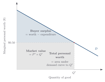
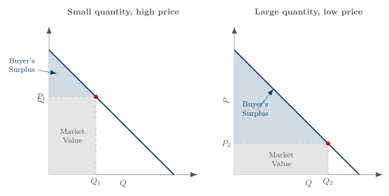
The surplus column also exposes a fallacy. A governor once defended cutting back farm labor because the smaller crop earned more revenue, so, he claimed, no harm was done. The error is treating revenue as welfare. Read down this demand schedule: market value rises, peaks, and falls as quantity grows, but total personal worth and consumer surplus rise throughout. A smaller crop can bring more revenue while leaving buyers with less total worth and surplus. That refutes the claim that no one was harmed. Judging growers and buyers together also requires production costs and the distribution of revenue. Revenue alone cannot answer the welfare question.

Demand Is a Rate, Not a Pile

A small but stubborn confusion: demand describes a rate of consumption, a flow over time, not a fixed lump. The milk schedule is quarts per week, and the unit matters: consumption is a rate even when the good sits around as a stock. The milk in your refrigerator is a stock on hand, the quarts you drink per week is the rate, and demand is about the rate.

Because demand is a rate, not a weekly delivery slip, you cannot read a year’s demand as a fixed weekly quota. If a household’s demand for water doubles over a year, from roughly 3,650 to 7,300 gallons, you cannot say how many extra gallons fall in the first week. The rate is what doubles; the week-to-week timing floats around it.

A Price Is an Exchange Rate, and It Can Exist Without Money

Underneath every dollar figure is something more basic. A price is an exchange rate between goods, how much of one thing you give up for another. Money is just one good we happen to quote prices in, which means prices can exist with no money at all. Picture children swapping snacks at lunch, or a disaster zone where cash has stopped circulating: a bottle of water might trade for three granola bars, and that granola-per-bottle rate is a real price, every bit as binding as a dollar tag. So the price that actually governs your choices is the relative price, what a good costs in terms of other goods, not its dollar tag in isolation. We will lean on that idea heavily when we take up elasticity and its applications next.

There Is No Such Thing as a Fixed Need

Now we can separate two meanings of the slippery word from the opening. Biology and engineering can identify quantities required for a specified outcome, such as calories needed to avoid a defined deficiency. Economics asks a different question: how much of a scarce good people choose or a policy supplies when obtaining more sacrifices alternatives. The amount of any good a person or a society chooses is a function of its price. That shorthand needs care: choices also depend on income, rights, information, and other conditions, while a social total aggregates individual choices. A need label alone cannot answer how much at what price.

To see the choice claim, picture someone with almost nothing, down to bare necessities. Within a feasible voluntary choice set, a little more food can be traded against some clothing, and enough of another comfort can make parting with a little food worthwhile. Safety also enters trade-offs: people accept small increments of risk when driving faster or pursuing other goals. These examples do not deny deprivation or coercion; they show that chosen margins are comparisons rather than all-or-none labels.

Political need-language misleads when it makes a quantity sound settled without stating an outcome, cost, distribution, or alternative. Calling a good necessary may be a defensible value judgment or policy priority, but it does not reveal how much more is worth obtaining or who should bear the sacrifice. The label begins that argument; it does not finish it.

A bonus from taking the point seriously: demand reasoning reaches beyond store prices. Family size, migration applications, medical procedures, and other choices can respond to a full price that includes time, risk, legal constraints, and forgone alternatives. The prediction requires that price to be identified and other demand conditions held apart; a raw correlation is not by itself a demand-curve estimate.

For Further Reading

Want to explore the source material? This lecture draws on the following chapters from two books by Armen A. Alchian and William R. Allen:

• Universal Economics (Liberty Fund, 2018): Ch. 5, “Demands and the Laws of Demand”.
• Exchange and Production, 3rd ed. (Wadsworth, 1983): Ch. 2, “Consumer Demand”.