Who Really Pays? Taxes, Subsidies, and Elasticity

In October 2022 Florida cut its gasoline tax by 25.3 cents a gallon for one month. Drivers never hand that tax to the state; fuel suppliers pay it when the fuel leaves the terminal, and the pump price includes it. So here is the question that drives this post: of the 25.3 cents, how many reached drivers? All of them? None, because stations kept the savings? Some, and if some, what decides how many?

The same question applies to every tax, subsidy, and tariff. The law names who sends the money to the government, or who receives the check. Economics asks who ends up with less money, or more, once buyers and sellers have adjusted. You will answer it with the supply and demand tools from earlier in the course, on one running example, and return to Florida at the end.

A Tax Opens a Wedge, and the Price Rises by Less Than the Tax

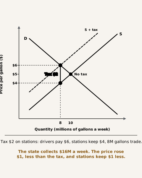
Suppose this is a weekly gasoline market. With no tax, drivers buy 10 million gallons a week and stations offer 10 million, at a price of $5 a gallon. The demand curve says that each $1 rise in the price cuts the amount drivers want by 2 million gallons. The supply curve says that each $1 rise in the price a station keeps raises the amount stations offer by 2 million gallons. We use a big $2 tax so the arithmetic is easy to see; a 25-cent tax works the same way.

Now the state collects a $2 tax from stations on every gallon they sell. A station that needed $5 to supply a gallon before now needs $7, because $2 goes to the state. Every point on the supply curve moves up by $2.

Try the obvious answer first: stations raise the price by the full $2, to $7. At $7 drivers want only 6 million gallons. Stations, keeping $5 of each $7 sale, are willing to supply 10 million gallons. So 4 million gallons sit unsold. Stations with unsold gasoline cut their price until drivers buy exactly what stations offer. That happens at $6: drivers want 8 million gallons, and stations, keeping $4 after the tax, offer 8 million.

So drivers pay $6, which is $1 more than before. Stations keep $4, which is $1 less. The quantity falls from 10 million to 8 million gallons. And the state collects $2 on each of 8 million gallons, or $16 million a week, half of it from each side. Stations wrote the whole check, but they passed on only half of it, because drivers buy less when the price rises.

The same split appears in Alchian and Allen’s 10-cent gasoline tax example, a short-run result: the price drivers paid rose by 3 cents and the price sellers kept fell by 7 cents. The tax neither stayed with the seller who sent it in nor passed entirely to the buyer. How it split depends on something other than the law. The next two sections show what.

Who Writes the Check Does Not Decide Who Pays

Change one thing. Suppose the law now makes drivers hand the $2 to the state at the pump, and stations keep every dollar they charge. Does the outcome change?

A driver who would have paid a station $10 for the first gallon now offers at most $8 to the station, because $2 goes to the state. Every point on the demand curve, as stations see it, drops by $2. That lower demand curve crosses supply at 8 million gallons and a station price of $4. Drivers pay the station $4 and the state $2, a total of $6. The numbers are identical: drivers pay $6 in all, stations keep $4, 8 million gallons trade, and the state collects $16 million.

Taxing the seller shifts supply up by $2; taxing the buyer shifts demand down by $2. Both open the same $2 wedge at the same quantity, so both give the same prices. The law picks who mails the check, not who bears the tax. That is why “make the companies pay” and “make the customers pay” can be one policy in disguise.

Could a law forbid stations to pass the tax on? It would work poorly, because stations have many other ways to pass on a cost. A station could, for example, raise the price of the drinks in its cooler. Block a cost at one place and it finds another way through, like water around a plugged hole in a dam. This repeats the lesson of the price-controls post.

Payroll taxes show the same thing in your own paycheck. By law, the Social Security and Medicare payroll taxes are split evenly. Workers pay 6.2 percent for Social Security and 1.45 percent for Medicare, a total of 7.65 percent of wages up to a yearly cap, and employers pay another 7.65 percent (IRS Topic 751). Does that mean workers bear only half of the tax? The wedge analysis says the legal split tells you nothing about the economic split. What matters is which side can more easily get out of the tax. An employer can hire fewer people and use machines instead, while a worker who lives on labor income has few ways to stop working. If employers can avoid the tax more easily, workers bear most of both halves. We return to labor markets later in the course; for now, the stub on your paycheck describes the law, not the incidence.

The Side That Cuts Back Less Bears More

If the legal payer does not decide the split, what does? Go back to the wedge. The tax opens a $2 gap between what drivers pay and what stations keep, and the market moves the price until drivers buy exactly what stations supply. Along the way, each side backs away from the trade to some degree: drivers buy fewer gallons because the price rose, and stations offer fewer because they keep less. The side that backs away more easily can push the burden onto the side that cannot.

Economists measure this backing away with elasticity: how much the quantity responds when the price changes. A side that cuts back a lot is elastic; a side that cuts back little is inelastic. The less elastic side bears more of the tax.

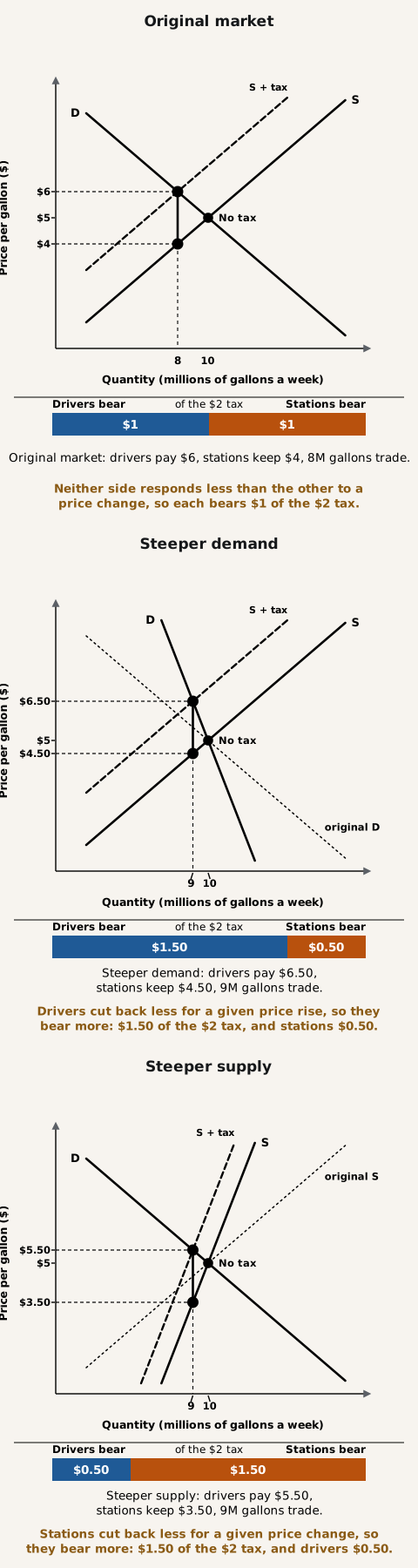
First suppose drivers cut back less than before. In the short run, many drivers cannot switch cars, move closer to work, or change their routes, so demand for gasoline is steeper. Keep the same starting point, $5 and 10 million gallons, but let demand be steeper through that point. Now the $2 tax gets a different result: the market settles at 9 million gallons, drivers pay $6.50, and stations keep $4.50. Drivers bear $1.50 of the $2 and stations only $0.50. Drivers keep buying nearly as much when the price rises, so stations can raise it by more.

Now suppose stations cut back less. In the short run, stations already have their tanks and pumps in place, so they will sell almost as much even if they keep less per gallon. Draw supply steeper through the same point, with demand as in the original market. The same $2 tax now leaves 9 million gallons traded, drivers paying $5.50, and stations keeping $3.50. Drivers bear only $0.50, and stations bear $1.50. The dime tax above, with sellers taking 7 cents of 10, belongs to this family.

Same $2 tax, same starting point	Drivers pay	Stations keep	Drivers bear	Stations bear
Original market	$6.00	$4.00	$1.00	$1.00
Drivers cut back less (steeper demand)	$6.50	$4.50	$1.50	$0.50
Stations cut back less (steeper supply)	$5.50	$3.50	$0.50	$1.50

In every row the two bearing columns add to $2. The tax is the same in all three; the market’s responsiveness changes who pays it. Where neither side cuts back less, the split is even. Where drivers do, they bear three-fourths; where stations do, stations bear three-fourths.

The limiting case is a good whose quantity cannot change at all. Suppose a city has uniform land that rents for $1.00 a square foot a month and levies a 40-cent monthly tax on it. The supply of land is a vertical line, since no more can be produced and none will disappear whatever the rent. Users’ demand for land has not changed either, so the rent they pay stays at $1.00. The owner, who used to keep $1.00, now keeps 60 cents. If an owner tries to charge more to recover the tax, the land goes unrented, and the rent falls back. A tax on pure land falls entirely on its owner, and it makes no difference whether the law makes the owner or the renter send in the 40 cents. Land is the extreme case, not the typical one: some land can be created, for example by filling in shoreline, and owners can often shift land between uses. The nearer a base comes to the extreme, the more fully the owner bears the tax.

A Tax Costs More Than It Raises, and the Gap Is the Trades It Blocks

So far we have asked who pays. Now ask what the tax costs them. We need a way to measure what trade is worth to each side.

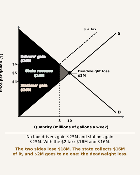
Most gallons are worth more to the driver who buys them than the $5 price; the first gallon is worth as much as $10 to some driver. The drivers’ gain from buying is the area between the demand curve and the price they pay. With no tax, that area is a triangle with a base of 10 million gallons and a height of $5, from the $10 the first gallon is worth down to the $5 price. Its area is one-half times 10 million times $5, or $25 million a week. The same logic gives stations’ gain from selling, the area between the price and the supply curve: also $25 million a week.

Now impose the $2 tax with the original curves. Drivers’ triangle shrinks to a base of 8 million gallons and a height of $4 (from $10 down to the $6 they pay), so their gain falls to one-half times 8 times $4, or $16 million. Stations’ gain, with a base of 8 and a height of $4 (from the $4 they keep down to the zero-cost first gallon), also falls to $16 million. Drivers lose $9 million and stations lose $9 million, a total of $18 million a week.

Where did the $18 million go? The state collected $16 million of it. That money is a transfer from buyers and sellers to the state, not a loss in itself. The other $2 million went to no one. It is the deadweight loss: the value of the 2 million gallons that no longer trade. Those gallons were worth more to drivers than they cost stations to supply, so the tax stopped trades that would have made both sides better off. Drawn on the supply and demand diagram, it is the small triangle with a base of $2 (the wedge) and a height of 2 million gallons, one-half times $2 times 2 million, or $2 million.

The amount lost depends on elasticity as well. In the steeper-demand market, the same tax leaves 9 million gallons traded. The state collects $2 times 9 million, or $18 million, and the deadweight loss is one-half times $2 times 1 million, or $1 million. The steeper-supply market gives the same figures. Tax something that people keep buying and you raise more money and block fewer trades; the more either side can cut back, the more trades the tax destroys and the less it raises.

$2 tax	Original market	Steeper demand	Steeper supply
Gallons traded after the tax	8 million	9 million	9 million
Revenue to the state	$16M	$18M	$18M
Deadweight loss	$2M	$1M	$1M

This is why a tax on land blocks no trades at all and a tax on gasoline blocks few. A tax on restaurant meals in one town on a state line, or on one theme park with rivals nearby, blocks many: diners and visitors simply go elsewhere, and the tax raises little. A state that wants revenue while blocking few trades taxes the base that cuts back least.

One caution before we leave the tax. The deadweight loss we measured is the loss in this market, with no other problem present. If gasoline use also imposes harms, such as pollution or congestion, that the price does not include, a tax can correct part of that problem instead of only creating a loss. The wedge diagram alone cannot tell you which case applies. Nor can it say who finally gains, because that depends on what the $16 million buys.

A Subsidy Is a Tax Run Backward, and It Costs More Than It Gives

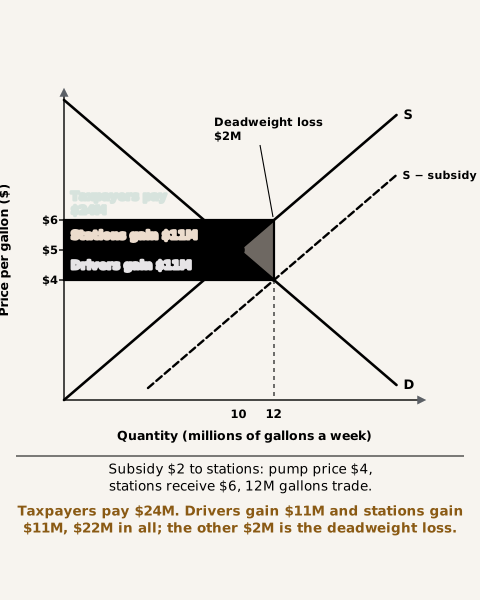
A subsidy is a payment to buyers or sellers for each unit traded, a tax with the sign reversed. Suppose the state pays stations $2 for every gallon they sell, so a station will now offer any amount for $2 less than before. The whole supply curve shifts down by $2.

Stations compete for drivers until the pump price falls to $4. A station selling at $4 and collecting $2 from the state receives $6. At those prices drivers want 12 million gallons, and stations, receiving $6, offer 12 million. Drivers gain $1 on each gallon and stations gain $1 on each gallon, and 12 million gallons trade instead of 10 million.

The state pays $2 on 12 million gallons, or $24 million, and the money comes from taxpayers. Compare that cost with what it buys. Drivers’ gain rises from $25 million to $36 million, up $11 million. Stations’ gain also rises from $25 million to $36 million, up $11 million. The two sides gain $22 million in all. Taxpayers pay $24 million and the market delivers $22 million, so $2 million is lost. The subsidy pushes trade past the point where the extra gallons are worth what they cost. The 2 extra million gallons cost stations between $5 and $6 to supply, but they are worth only between $5 and $4 to drivers. Those trades happen, but they are worth less than they cost, and the difference is the deadweight loss.

As with the tax, who gets the subsidy does not depend on who receives the check, and it goes more to the side that cuts back less. If drivers cut back less, as with steeper demand, drivers capture more of a subsidy given to stations. The pattern is the same as the tax, with the sign reversed.

The fixed-supply case shows this sharply. Suppose a neighborhood has 100 apartments, no more can be built soon, and rent is $3,000 a month. The city gives every renter a voucher worth $500 a month. Renters are now willing to pay owners $500 more for each apartment, but the supply of apartments is a vertical line, so owners cannot offer more. The rent that fills exactly 100 apartments rises from $3,000 to $3,500. Each renter still pays $3,000 out of pocket, because $500 of the rent is covered by the voucher. The owners capture the whole $500. A subsidy aimed at one group goes to whoever cannot adjust.

One caution: if the good also gives benefits to people outside the trade that its price leaves out, a subsidy may be justified. A later topic takes up that case. Without such benefits, a subsidy costs taxpayers more than it delivers.

The Law Picks Who Writes the Check; Elasticity Picks Who Pays

The model predicts that the side that cuts back less gets the larger share, whatever the law says. Researchers have checked this in several markets. The studies below are observational, so each is evidence consistent with the model, not a proof, and estimates vary across studies, places, and years.

Gas-tax holidays. In 2022 several states suspended their gasoline taxes for a time. A Penn Wharton Budget Model policy brief (He and Sun, June 2022) looked at three states. It estimated that drivers received about 72 percent of the tax cut in Maryland, between 58 and 65 percent in Georgia, and between 71 and 87 percent in Connecticut, and it noted that the price reductions were often not sustained for the whole holiday. In the short run, drivers cannot easily switch away from gasoline, so the model predicts that they would get most of a cut, and that is roughly what the estimates show. The brief is an early policy analysis, not a peer-reviewed study, and crude-oil prices were also moving.

Student loans. Lucca, Nadauld, and Shen (New York Fed Staff Report 733) studied federal loan limits. They found that a rise in the limit on subsidized loans was followed by tuition increases of about 60 cents for each additional dollar. The law names students as the beneficiaries. But if schools cannot quickly expand, for instance because new instructors are hard to train, their supply is inelastic, and the model predicts that they capture part of the subsidy. The size of this effect varies across studies and types of school.

Housing vouchers. Susin (2002) estimated that in the 90 biggest metropolitan areas, vouchers raised rents by 16 percent on average. The housing stock is nearly fixed in the short run, so supply is close to the vertical line in the apartment example, and a voucher that lifts what renters can pay pushes up the rent.

Tariffs. A tariff is a tax on imports, paid by the importer when goods cross the border. Amiti, Redding, and Weinstein (2019) studied the U.S. tariffs of 2018. They found that foreign sellers did not cut their prices, so the full tariff showed up in the prices of imported goods in the United States, and the burden fell on U.S. buyers and importers. One reading is that foreign sellers could sell the goods to other buyers while U.S. buyers had few quick substitutes, which the model says leaves the burden with buyers. Note that this result concerns prices at the border, not the prices on store shelves.

Now go back to Florida. The state cut the tax by 25.3 cents for October 2022, and the tax is collected from suppliers at the terminal. Whether the cut reached drivers depended on how easily drivers and stations could back away from trading. We do not have a reliable estimate for Florida’s own holiday. In the three states above, drivers got between 58 and 87 percent of the cut, though the price drops often faded before the holiday ended. A tax cut is the same wedge run backward: the pump price falls by the drivers’ share of the cut, and the rest stays with the sellers. Compare your opening guess with those ranges, and ask what it assumed about who cuts back less.

For Further Reading

Want to explore the source material? This lecture draws on the following chapters from two books by Armen A. Alchian and William R. Allen:

• Universal Economics (Liberty Fund, 2018): Ch. 17, “Timing of Adjustments”.
• Exchange and Production, 3rd ed. (Wadsworth, 1983): Ch. 4, “Market Prices as Social Coordinators”.