Present Value and the Interest Rate

Almost every decision worth making spans time. You spend money now to earn a degree that pays off for decades. A firm builds a factory this year to sell goods for years. A government borrows today and taxes tomorrow. In all of these, costs and benefits land at different dates, which raises a problem we have so far ignored: how do you compare a dollar today with a dollar next year, or thirty years from now? You cannot just add them up. A thousand dollars promised long ago and a thousand dollars in your pocket today are not the same thing, and treating them as equal is one of the most common and expensive mistakes people make.

This topic gives you the tool that solves it. It is called present value, and it puts amounts arriving at different times onto a single ruler so they can be compared. This is the capitalization tool the course has been promising since T7, when future profit first got baked into today’s asset price. Out of that one idea comes a surprising amount: what interest really is and where it comes from, how to price a loan, and why a future payment is worth less than a present one. We build the arithmetic first in this post, then point it at durable assets, your own earnings, and profit in the next. Everything here is one tool used over and over; state it clearly now and the rest of the topic falls out of it.

A Future Dollar Is Worth Less Than a Present Dollar

Start with the most basic move. If you put $100 in an account paying 6 percent a year, in a year you have $106. The rate of interest is the rate at which that present amount grows into a future one. Write it as a formula and the whole topic unfolds from it:

P × (1 + r) = F

Here P is the present amount, r is the interest rate, and F is the future amount. With P = $100 and r = 0.06, F comes out to $106. This forward direction, present to future, is compounding: each year’s interest itself earns interest, so growth does more than beginners expect. The table below shows what $1 grows to over time at various rates. Read it as a multiplier: at 7 percent for ten years, $1 becomes $1.97, so $350 becomes about $690.

Future value of $1 (what a present $1 grows to). Selected rates and years.

Years	3%	4%	5%	6%	7%	8%	10%	12%	15%	20%
1	1.03	1.04	1.05	1.06	1.07	1.08	1.10	1.12	1.15	1.20
3	1.09	1.13	1.16	1.19	1.23	1.26	1.33	1.41	1.52	1.73
5	1.16	1.22	1.28	1.34	1.40	1.47	1.61	1.76	2.01	2.49
10	1.34	1.48	1.63	1.79	1.97	2.16	2.59	3.11	4.05	6.19
15	1.56	1.80	2.08	2.40	2.76	3.17	4.18	5.47	8.14	15.41
20	1.81	2.19	2.65	3.21	3.87	4.66	6.73	9.65	16.37	38.34
30	2.43	3.24	4.32	5.74	7.61	10.0	17.4	30.0	66.21	237.4

A couple of entries are worth noting. Put $250 in at 7 percent for three years and you have about $306 ($250 × 1.23). And notice how fast money doubles: at 5 percent, $1 grows past $2 in about fourteen years; at 10 percent, in about seven. That regularity has a handy shortcut called the Rule of 72: divide 72 by the interest rate and you get the rough number of years it takes money to double. At 7 percent, 72 ÷ 7 is about ten years. At 12 percent, about six — a good enough approximation to do in your head.

Compounding also explains how modest-looking sums become large. A piece of land bought for $5,000 and worth $85,000 thirty years later has grown seventeenfold; the table implies a compound growth rate of about 10 percent. The same arithmetic can describe rabbits multiplying or grain planted and harvested, although a physical growth rate becomes an economic return only after valuing all inputs, outputs, and costs. Whenever a value compounds at a steady percentage, the formula tells you how a present amount maps into a future one.

Present Value Reverses the Arithmetic

Now run the formula backward. For otherwise comparable, certain amounts and a positive rate, an amount arriving in the future has a smaller present value. Recover it by dividing instead of multiplying:

P = F ÷ (1 + r)

Take $220 due one year from now at 10 percent. Its present value is $220 ÷ 1.10 = $200. The future $220 has been discounted to a present value of $200. The discount factor is 1 ÷ (1 + r); here it is 0.909. This operation puts amounts dated at different times on one common date. The rate must fit the comparison: different risk, liquidity, taxes, or contractual terms can require different rates.

The table below gives the discount factors directly: the present value of $1 received after the listed number of years (simply the reciprocals of the table above).

Present value of $1 (today’s value of $1 received in a future year). Selected rates and years.

Years	3%	4%	5%	6%	7%	8%	10%	12%	15%	20%
1	0.97	0.96	0.95	0.94	0.94	0.93	0.91	0.89	0.87	0.83
3	0.92	0.89	0.86	0.84	0.82	0.79	0.75	0.71	0.66	0.58
5	0.86	0.82	0.78	0.75	0.71	0.68	0.62	0.57	0.50	0.40
10	0.74	0.68	0.61	0.56	0.51	0.46	0.39	0.32	0.25	0.16
15	0.64	0.56	0.48	0.42	0.36	0.32	0.24	0.18	0.12	0.07
20	0.55	0.46	0.38	0.31	0.26	0.22	0.15	0.10	0.06	0.03

Two patterns in this table are themselves economic lessons. First, hold the rate fixed and read down a column: the farther into the future an amount lies, the smaller its present value. At 4 percent, $2,500 due in five years is worth $2,500 × 0.82 = $2,050, but the same $2,500 due in ten years is worth only $2,500 × 0.68 = $1,700. Distance in time eats into value, because over a longer wait, a smaller present sum could have grown to the target on its own. Second, hold the year fixed and read across a row: the higher the interest rate, the smaller the present value. That same $2,500 in five years is worth $1,950 at 5 percent but only $1,700 at 8 percent. A higher rate discounts future amounts more heavily.

Suppose someone offers either $30,000 in ten years or $40,000 in fifteen years. Which is better? It depends on the applicable rate. At 6 percent their present values are both about $16,800; at 4 percent the later prize pulls ahead. Reduce each comparable alternative to present value so both sit on the same date. A $1,000 college loan carrying no interest and repaid years later is partly a subsidy if its risk-adjusted market rate would be positive: the repayment’s present value is then less than $1,000.

Interest Is the Price of Current Income, Set Where Saving Meets Investment

We have used the interest rate as a given. Where does it come from, and why is it positive at all?

Two forces organize the benchmark. The first is the productivity of investment. Resources set aside and put to work can yield more later: grain planted can yield a larger harvest, and grapes can become wine worth more than the juice after all costs. Investing means giving up some consumption now in pursuit of more value later. Painting your house instead of spending the weekend gaming is an investment if the preserved house is worth the sacrificed time and materials.

But not every roundabout, time-consuming method pays off. The claim that “more roundabout production is always more productive” is false. Only the right methods in the right amounts add to wealth. So the productivity of investment is real but not automatic.

The second force is time preference: holding amount and certainty fixed, people may prefer consumption sooner rather than later. Uncertainty is separate. A risky promise can require a default or risk premium even for someone with no pure impatience; Part B decomposes the observed rate package.

Put these together in a market and the interest rate is a price like any other: the price of current income in terms of future income. People who want current income to invest or consume demand it; people willing to exchange current income for more future income supply it. In a simple competitive, closed-economy loanable-funds model, their plans meet at a market-clearing rate. If $100 today trades for a comparable, certain promise of $105 next year, the rate is 5 percent: r = (105 − 100) ÷ 100.

In that model, a lender buys a claim to future income and a borrower sells one for resources now. Demand for current income slopes down because more projects clear a lower hurdle rate. The diagram draws saving upward-sloping: a higher rate induces more saving, holding wealth and expectations fixed. That is a maintained baseline, not a universal individual response; income effects can offset substitution, and international capital flows can shift market supply.

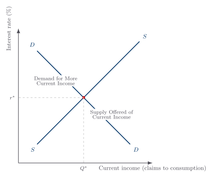
Consumption and investment borrowing both press on credit markets. Although realized saving and investment are linked in national accounting, planned saving and planned investment can differ. Banks, bond markets, equity markets, retained earnings, and international flows help coordinate them; the diagram compresses that network into one price-and-quantity model.

One warning: interest is not simply “the price of money.” Observed nominal rates price claims across time and can include expected inflation, default, term, liquidity, and administrative components. Monetary policy can affect market rates through several channels, but that macroeconomic analysis is outside this course. Part B handles the rate package needed for microeconomic comparisons.

An Annuity Is a Stream, and a Perpetuity Lasts Forever

Most real decisions involve not a single future amount but a stream of them: a pension, a loan repaid in installments, a building that throws off rent for decades. A level stream of equal annual payments is an annuity. Its present value is just the sum of the discounted individual payments, but summing a column of discount factors by hand is tedious, so we tabulate the totals. The table below gives the present value of $1 received at the end of each year for the listed number of years, an annuity factor: multiply it by the annual payment to get the whole stream’s present value.

Present value of $1 received at the end of each year (annuity factors). Selected rates and years.

Years	3%	4%	5%	6%	7%	8%	10%	12%	15%	20%
1	0.97	0.96	0.95	0.94	0.94	0.93	0.91	0.89	0.87	0.83
3	2.83	2.78	2.72	2.67	2.62	2.58	2.49	2.40	2.28	2.11
5	4.58	4.45	4.33	4.21	4.10	3.99	3.79	3.61	3.35	2.99
10	8.53	8.11	7.72	7.36	7.02	6.71	6.15	5.65	5.02	4.19
15	11.94	11.12	10.38	9.71	9.11	8.56	7.61	6.81	5.85	4.68
20	14.88	13.59	12.46	11.47	10.59	9.82	8.51	7.47	6.26	4.87
30	19.60	17.29	15.37	13.77	12.41	11.26	9.43	8.06	6.57	4.98

This one table does enormous work. A three-year annuity of $1,000 at 8 percent is worth $1,000 × 2.58 = $2,580. If your rich uncle buys you fifteen years of $50,000 a year, beginning next year, at a 10 percent rate the stream is worth about $380,500 today, not the $750,000 eventually paid. That is not a contradiction: $750,000 is the nominal sum of payments, while $380,500 is their value at one date under the stated rate. The factor also runs in reverse. If $500,000 today finances a fifteen-year level stream at 10 percent, it supports about $65,700 a year. Given a market price and promised payment, search the table to recover the implied rate. Then ask whether default risk, fees, taxes, timing, or other contract terms make that rate comparable to the alternative you care about.

The same machinery prices an ordinary loan, and it clears up something most borrowers never notice. Taking out a mortgage or car loan repaid in equal yearly (or monthly) installments means selling the lender an annuity: the loan amount is the present value, and the level payment is whatever annual figure makes that stream’s present value equal the sum you borrowed. Run the annuity table in reverse to find it. Borrow $80,000 over twenty years at 5 percent, and the twenty-year, 5 percent annuity factor (about 12.46) says the level payment is roughly $80,000 ÷ 12.46, about $6,400 a year.

Every one of those level payments splits into two pieces, interest on the balance still owed plus a repayment of principal, and the mix shifts over the life of the loan. Early on, you owe a lot, so most of the payment is interest and little goes to principal; as the balance falls, the interest piece shrinks and more of each payment chips away at principal. Your equity, the part of the asset you actually own free and clear, therefore builds slowly at first and then accelerates. The table below traces the first two years of that $80,000 loan.

How a level loan payment splits into interest and principal (first two years). $80,000 borrowed at 5%, level payment $6,400/year.

Year	Balance owed at start	Interest (5% of balance)	Principal repaid (payment − interest)	Equity built this year
1	$80,000	$4,000	$2,400	$2,400
2	$77,600	$3,880	$2,520	$2,520

In the first year, $4,000 of the $6,400 payment just covers interest, leaving $2,400 to build equity. In the second year, you owe less ($77,600), so interest falls to $3,880 and $2,520 of the same payment goes to principal. The payment never changes, but its composition does, which is why equity builds faster over time. It is the present-value arithmetic of an annuity, read one year at a time.

Streams need not be level. When the yearly amounts vary, you discount each separately and add. The next table works a six-year stream at 8 percent. Multiply each future amount by its discount factor, then sum the present-value column.

Present value of a six-year varying annuity at 8%.

Year	Future amount	Discount factor (8%)	Present value
1	$1,000	0.926	$926
2	$2,000	0.857	$1,714
3	$3,000	0.794	$2,382
4	$3,000	0.735	$2,205
5	$2,000	0.681	$1,362
6	$1,000	0.630	$630
Total			$9,219

This table delivers a deeper lesson: market value can change when expectations change, before the future cash arrives. If news doubles expected receipts in years five and six to $4,000 and $2,000, the calculated present value jumps from $9,219 to $11,211, assuming the rate and other expectations stay fixed. Part B uses that capitalization mechanism for policy and profit.

Now stretch the stream out forever. An annuity that pays a constant amount in every future year, without end, is a perpetuity, and it has a simple value:

P = A ÷ r

The present value of a perpetuity is just the annual amount divided by the interest rate. A perpetuity of $1 a year at 5 percent is worth $1 ÷ 0.05 = $20. That seems impossibly small for an endless stream, until you see why: invest $20 at 5 percent, collect the $1 of interest each year, spend it, and the $20 is still there to repeat the trick forever. The distant future barely adds anything, because those far-off dollars are discounted to almost nothing. The next table makes this concrete by splitting a perpetuity into its first fifty years and everything after.

How much of a perpetuity’s value comes from the distant future.

Interest rate	Present value of first 50 years	Present value of year 51 onward	Present value of entire perpetuity	Share beyond year 50
3%	$25.70	$7.30	$33.33	about 22%
5%	$18.30	$1.70	$20.00	about 8.5%
10%	$9.91	$0.09	$10.00	under 1%

At 10 percent, everything beyond the first fifty years is worth nine cents on a ten-dollar claim. The distant share is much larger at lower rates, which is why the chosen rate matters greatly for long-lived consequences.

Interest Is a Cost Even When You Never Borrow

A costly mistake is thinking that if you do not borrow, waiting has no cost. Interest is the cost of waiting: the cost of having something later rather than sooner when the relevant rate measures the return on the best comparable alternative.

Suppose a venture spends $1,000 at the start of year one and collects $1,300 at the end of year two, with nothing left over. Is it profitable? You cannot just subtract $1,000 from $1,300 and declare a $300 profit, because those amounts sit two years apart. You have to capitalize both to a common date using the interest rate. The table below values everything at both dates, start and end, with the same result.

Capitalizing costs and receipts to a common date, at a 7% interest rate.

	Capitalized to start of year 1	Capitalized to end of year 2
Outlay ($1,000 at start of year 1)	$1,000	$1,000 × 1.07 × 1.07 = $1,145
Receipts ($1,300 at end of year 2)	$1,300 ÷ (1.07 × 1.07) = $1,136	$1,300
Result	$1,136 − $1,000 = $136 profit	$1,300 − $1,145 = $155 profit

At a 7 percent opportunity-cost rate the venture earns a profit; $136 and $155 are the same value difference measured at different dates. At a 15 percent rate it becomes a loss:

The same venture at a 15% interest rate.

	Capitalized to start of year 1	Capitalized to end of year 2
Outlay ($1,000 at start of year 1)	$1,000	$1,000 × 1.15 × 1.15 = $1,322
Receipts ($1,300 at end of year 2)	$1,300 ÷ (1.15 × 1.15) = $983	$1,300
Result	$983 − $1,000 = $17 loss	$1,300 − $1,322 = $22 loss

No money was borrowed, yet using the firm’s own cash still forgoes another use. The relevant hurdle is the expected return on a comparable alternative, adjusted for risk and other differences, not automatically any advertised loan rate. A lottery can truthfully total $1,000,000 in nominal payments while having a present value below $1,000,000. Discounting costs and receipts to one date makes them comparable; the economic judgment still depends on the cash-flow forecast and chosen rate. Part B connects that comparison to profit.

For Further Reading

Want to explore the source material? This lecture draws on the following chapters from two books by Armen A. Alchian and William R. Allen:

• Universal Economics (Liberty Fund, 2018): Ch. 30, “Arithmetic of Capital Values”; Ch. 31, “Series of Future Values and Annuities”; Ch. 36, “Determinants of the Interest Rate”.
• Exchange and Production, 3rd ed. (Wadsworth, 1983): Ch. 6, “Capital Values, Future Yields, and Interest”; Ch. 16, “Wealth: Saving and Investing”.