Factor Markets and Labor, Part A: What an Extra Worker Is Worth

So far we have studied the buying side of the economy: how people choose what to consume, how prices ration scarce goods, how trade leaves both sides better off. Now turn the picture around. The same people who buy groceries also sell something to earn the money that buys them. Most of us sell our labor; some also sell the use of land, machines, or savings. These are the factors of production, the inputs firms hire to make everything else, and the markets where they get hired and priced are factor markets.

A huge amount of public argument turns on these markets. Why does a surgeon earn more than a cashier? Why does the same job pay differently in different countries? Are CEO salaries proof the market has gone haywire? Is “the rich get richer, the poor get poorer” a fair description of how incomes move over a lifetime? Every one of these questions turns on a single idea we will build from scratch here: the value of what an extra worker adds. Get that straight and the rest falls into place.

This is the first of two parts. Here in Part A we build that central idea and use it to explain how labor demand works, why “machines destroy jobs” is mostly a confusion, and why people’s earnings differ. Part B takes the same engine into the most heated policy fights of all: unions, the minimum wage, discrimination, and occupational licensing.

Labor Is Wanted for What It Helps Produce, Not for Itself

Nobody hires a worker for the pleasure of his company. A firm hires labor because labor helps produce something customers will pay for. Economists say the demand for any input is a derived demand: it is derived from the demand for the product the input makes. There is no demand for autoworkers apart from the demand for cars, no demand for cooks apart from the demand for meals.

This quietly settles a great deal. It means the value of a worker is not a fixed personal trait you carry around like your height. It depends on what that worker helps produce and what people will pay for it. The same person can be worth far more in one setting than another. Drop a skilled mechanic into an economy with no tools, no reliable transport, and no honest courts, and the value of his work collapses, not because he got worse but because the surroundings that turned his effort into valuable output disappeared. A worker’s productivity depends on the capital, the coworkers, the roads, even the level of corruption around him. So the same labor is worth different amounts in different places, which is most of why wages differ so much across countries.

When we ask “what is a worker worth,” then, we are really asking “how much does this worker add to what the firm can sell.” To answer that precisely we need a tool.

A Worker’s Pay Traces to the Value of What One More Worker Adds

Once you have the central construct, the policy questions almost answer themselves. Start with a puzzle about teams.

Working alone, Jack produces output worth $5 a day and Jill $7. Teamed up they produce $15, three dollars more than their solo sum, because they help each other.

	Output value
Jack, working alone	$5
Jill, working alone	$7
Jack and Jill together	$15

So how much did Jack add? Without him the team would have had only Jill’s $7, so Jack added $15 − $7 = $8. By the same logic Jill added $15 − $5 = $10. Those sum to $18, more than the $15 the team produced. Both numbers are correct, and they cannot both be paid. That is the catch with teamwork: the extra value from working together cannot be cleanly sliced and handed to one member. What pins down each person’s pay is not this impossible accounting but competition. A worker must be paid at least what he could earn on his next-best team elsewhere, and no more than he adds here.

To see how the value of an added worker drives hiring, we need a cleaner setting. Picture a small island, Codlandia. A thousand people live there, and at first everyone fishes from shore, catching 8 fish a day each. Then someone finds a boat, far more productive than the shore but with limited room, and that limit is what makes the example work. Here is the catch as more people climb aboard.

People on the boat	Total catch	Extra catch from the last person (marginal product)	Average catch per person
0	0	0	0
1	12	12	12.0
2	30	18	15.0
3	46	16	15.3
4	58	12	14.5
5	66	8	13.2
6	70	4	11.7
7	72	2	10.3
8	64	−8	8.0

The third column is the heart of the topic. The marginal product of a worker is the extra output the firm gets from adding one more, holding everything else fixed. The first person aboard adds 12 fish; the second adds 18, more than the first, because two can work the boat better than one. But after that the third adds 16, the fourth 12, the fifth 8. Past the second worker, each new person adds less than the one before. That is the law of diminishing marginal returns: as you keep adding one input to a fixed amount of others, the extra output from each new unit eventually falls. There is only so much boat, and crowding sets in.

Diminishing marginal returns is not the same as falling output. Through the seventh worker the total catch is still rising; it just rises in smaller steps. Total output turns down only once marginal product goes negative, at the eighth worker, who gets in everyone’s way and cuts the catch by 8. So a firm can keep gaining from added workers long after each adds less than the last.

This also fixes where a sensible employer operates. Nobody stops hiring in the rising stretch from the first to the second worker, where each adds more than the last; you would always want one more. And nobody hires into the region where an extra worker shrinks total output. A profit-seeker operates in the middle, the region of diminishing but still positive marginal product.

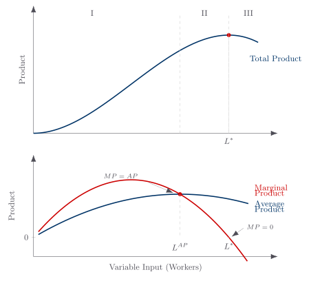
Put a price on the fish and the construct is finished. Suppose each fish is worth one unit. Then the marginal product column is also the value of marginal product (VMP): the extra output from one more worker, valued at what that output sells for. VMP is the demand for labor; it tells the employer the most each successive worker is worth paying.

People on the boat	Marginal product (fish)	Value of marginal product
1	12	12
2	18	18
3	16	16
4	12	12
5	8	8
6	4	4
7	2	2

Now the punch line, the hiring rule: hire each worker up to the point where the value he adds equals the wage you must pay him. A worker could catch 8 fish on shore, so to lure him aboard you must pay a wage of 8 fish. The owner keeps hiring as long as the next worker adds at least 8 in value. The fifth adds exactly 8, so the owner hires five and stops; a sixth would cost 8 to add only 4. Raise the wage and the calculus shifts: if shore fishing improves so the going wage is 12 fish, the owner hires only to the fourth worker, whose VMP is 12. A higher wage means fewer workers hired. That downward relationship is exactly why the demand curve for labor slopes down, and it falls straight out of diminishing returns.

Two results follow. First, VMP sets both how many to hire and what the input earns: in a competitive market a worker tends to be paid the value an added worker contributes, because paying less lets a rival bid him away and paying more loses the firm money. Second, the value left after the wage bill, the catch minus what the workers are paid, goes to the owner who supplied the boat and bore the risk. That residual is not a leftover slice of the workers’ product; it is the return to the boat and to the person who shouldered the chance the venture might fail. This is the same residual-claimant incentive we met in the property-rights and public-goods topic, now shown inside a production team. If the wage rose so high that paying it left the owner worse off than fishing on shore himself, he would beach the boat. Total factor payments cannot exceed the value produced, because any employer who tried would go broke, and competition steadily pushes payments toward the value each input adds.

That is the engine. The rest of the topic applies it to real arguments.

Higher Input Prices Push Firms to Substitute, and “Capital Replacing Labor” Hides the Labor Inside the Capital

The VMP picture has a second blade. When an input gets more expensive, firms do not just hire less of it; they shift toward other inputs that now deliver more value per dollar. A gardener whose wage doubles because fewer gardeners are available does not simply price himself into idleness. Homeowners switch to power equipment that lets one person do the work of several, or to rock gardens and low-maintenance plants. If you wonder what the substitutes for a costly input are, watch what its competitors sell: the makers of riding mowers and gravel will gladly show you.

This runs even when a firm seems locked into a fixed recipe. Suppose a tool needs exactly one handle per blade. Make handles costlier and the tool costs more; at the higher price consumers buy fewer tools, so fewer handles get used. The substitution happened, just out among the products rather than inside the factory. And these adjustments deepen over time, so demand for an input is more elastic in the long run than in the short run.

This sets up one of the most stubborn confusions in economics. People say a robot “substitutes capital for labor,” as if the machine made human work vanish. The robot, its software, and its sensors were all made by labor. What really happened is that the labor used to build the machine was substituted for the labor that used to do the task on site. The one-man bus is the cleanest case: a coin box and an automatic door replaced the conductor, but workers elsewhere had to make the coin box and the door mechanism, and the on-board labor that remains is reorganized into a higher-output job. Calling it “capital for labor” counts the labor you can see and ignores the labor embodied in the capital.

The same substitution logic explains a puzzle you might run into about public transit. Force bus drivers’ wages well above the market rate and a transit system does not simply pay up and carry on; it shifts the mix of inputs. Operators move to bigger buses run by fewer drivers, cut the number of routes, and stretch the gaps between buses, so riders wait longer. The expensive input gets economized on, here by substituting more capital and more rider waiting-time for the now-costlier driver labor, exactly as a homeowner trades a gardener for a riding mower.

There Is No Fixed Number of Jobs

The substitution point disposes of a fallacy that wrecks more public debate than almost any other: the belief that there is a fixed stock of jobs, so that every task a machine takes is a job permanently lost. Economists call this the lump-of-labor fallacy.

In a world of scarcity human wants are endless, so there is always more valuable work waiting than there are people to do it; only the highest-value jobs get filled at any moment. When a refrigerator eliminates the iceman’s route, or a household appliance eliminates the domestic servant, or a robot eliminates an assembly task, the freed workers do not evaporate. They move to the best of the still-unfilled jobs, very often including the jobs of building the new machines. The total number of jobs is not reduced, because the amount of work worth doing was never fixed. And the community ends up wealthier, because the same people now produce more.

A federal judge once stumbled here, ruling that a dispute over railroad layoffs had to come down “in favor of jobs,” as if the choice were between jobs and machines. But the real choice was between jobs and jobs: the railroad jobs on one side, and on the other the jobs displaced workers would take elsewhere, including jobs making railroad equipment. There is no contest between jobs and capital, because capital is itself made by labor and frees labor for other work.

One honest caveat: the fallacy is not that nobody is ever hurt. The community gains, and most workers gain from most innovations, but a particular worker displaced by a particular machine has no guarantee he personally comes out ahead from that specific change. The point is about the total. Automation does not shrink the pool of jobs while scarcity lasts; it reshuffles which jobs get done. That holds even for less-skilled work, since pushing a button often demands less skill than the craft it replaced.

Productivity Is Not Merit, and Technical Efficiency Is Not Economic Efficiency

Because labor is valued by what it produces, it is tempting to read high output as personal virtue and low output as failing. Resist that. Productivity reflects the whole package: the worker, yes, but also his tools, his teammates, and the institutions around him. A worker in a prosperous country often produces far more than an equally diligent worker in a poor one, not because he tries harder but because he works with better capital inside better institutions. Output measures value produced, not character. The same point explains why a firm sometimes leaves a low-wage country for a higher-wage one: the wage rate is only one part of the cost, and where better tools, reliable courts, and skilled coworkers raise total output enough, the higher-wage location can still be the cheaper place to produce.

A related trap: more physical output is not automatically “better.” One farm yields 30 bushels an acre, another 50. The second is not obviously superior until we ask what each crop cost to grow. If the high-yield land soaked up far more fertilizer, labor, and machinery, it may be the worse use of resources. A jet engine with more thrust per pound is not the better engine if it guzzles fuel to get there. A jet plane crosses the country hours faster than a propeller plane, yet which is more efficient cannot be read off the speed alone, because we have not been told what the speed costs. Efficiency compares the value of what you get against the cost of getting it; a bare physical ratio leaves out the cost side. This is the VMP idea from the output end: what counts is value net of cost, not raw quantity.

It pays to name the distinction these examples turn on, because it settles a long string of policy arguments. Technical efficiency means getting the most output from a given set of inputs, or, equivalently, using the least-cost combination of inputs to produce some stated output. It is a purely engineering test: no resources wasted in the making. Economic efficiency is a broader test that asks the question engineering cannot, namely whether the output is even worth what it cost. A reservoir dam can be technically efficient, built by the cheapest sound method, and still be economically inefficient if the water it stores is worth less than the resources sunk into impounding it. A steer bred to sell for half again as much per pound may or may not be the one to raise; the premium tells us nothing until we know what the fancy breeding cost. Technical efficiency can certify the method; only economic efficiency can certify that the project should be done at all.

Economic efficiency is the more general test for a precise reason. There are usually many technically efficient ways to do a thing, each wasting no inputs in its own terms; of those, only one minimizes the value of the opportunities you forgo to do it, and that one is the economically efficient choice. The broadest version of the idea even decides what to produce, not merely how cheaply to produce some arbitrary thing, by judging every output against what people will pay for it in exchange. That is why there are really two grades of economic efficiency. Cost minimization, finding the cheapest way to make a given output, is the narrower one; profit maximization is the more general, because it compares the value of what is produced against its cost, and so refuses to make cheaply a thing that is not worth making at all.

This is also why a great deal of official language about efficiency is empty. When a regulator says broadcast rights should be assigned to “permit maximum usage,” the instruction means nothing, because usage is not a single measurable dimension you can maximize. Told to “maximize the use” of one sheet of paper, you could not say what to do; the phrase can be made to mean anything. The sensible version is economic: assign the rights to whoever will get the most value from them relative to cost. The same flaw runs through standards that order up more of one favored quantity in isolation. When the government mandates that appliances hit a minimum output per kilowatt-hour, or that cars average a minimum miles per gallon, it minimizes a single input, energy, and drives up the others, the steel, plastics, engineering, and labor used to wring out the savings. Squeezing one input is not the same as minimizing total cost. These rules are almost certainly wasteful, because the resources spent to save the fuel are worth more in other uses than the fuel they save; if the trade were genuinely worth it, buyers would have chosen the thriftier product on their own.

Earnings Differ Because People and the Cost of Acquiring Skills Differ

Now we can explain why wages differ across people, not just countries. Two forces are at work, both flowing from VMP. People differ in their productive abilities, so they add different value. And people differ in the cost of acquiring the skills that raise that value. A surgeon earns more than an orderly partly because she adds more value and partly because few are willing or able to pay the long, costly price of becoming one, which restricts supply and props up the wage.

This gives a neat boundary. A wage gap between two jobs cannot stay much larger than the cost of acquiring the higher-paying skill. If it did, people would pour into the training, the added supply would push the wage down, and the gap would shrink to roughly what the training costs. So training cost works on both sides: it signals the value the trained worker can add, and it limits how many acquire the skill.

The same logic explains why we all teach ourselves to read, write, drive, and cook but hire out our medicine and our lawsuits. Generalized skills like reading are cheap to acquire, useful almost anywhere, and durable, so it pays each of us to own them. Specialized skills like surgery or tax law are expensive, narrow, and can lose value when the situation changes, so it pays to buy them from a specialist only when we need them.

Skills Are Wealth, and Unlike Property They Cannot Be Confiscated

It helps to think of skills as a form of wealth. Economists call it human capital: the productive capacity stored in a person through education, training, and experience. Like a machine, it took resources to build and yields a return over time. Unlike a machine, no one can take it from you.

That feature has a striking historical consequence. Where people have feared that physical property, land, shops, savings, could be seized by a hostile government or mob, they have tended to invest instead in portable professional skills, which travel in the head and survive across borders. The recurring pattern among persecuted minorities who built their security in medicine, law, scholarship, and trade reflects exactly this: human capital is the one form of wealth a persecutor cannot confiscate. That same insight ties human capital to discrimination, a thread Part B picks up directly.

Small Differences in Talent Can Produce Huge Differences in Pay

People point to enormous salaries, a CEO paid millions, a singer or athlete paid more than a thousand ordinary workers combined, as evidence that pay has come unmoored from contribution. Usually it has not. Two features of modern markets concentrate rewards on the very best, and both are consistent with VMP.

The first is scale. A giant firm’s CEO and a small firm’s manager may do recognizably similar work, yet the large-firm CEO earns vastly more, because a small edge in judgment applied across an enormous base of capital swings far more value than the same edge at a corner store. A decision one percent better is worth a fortune when it governs billions and pennies when it governs thousands. Pay scales with the stakes, not because the work is a thousand times harder.

The second is replicability. When a service can be delivered to millions at once, a recording, a broadcast, a piece of software, the slightly better performer serves the whole market, and a tiny edge in quality captures a giant share of the rewards. Fans want the best singer, and a recording lets that one singer reach everyone, so the second-best earns a fraction despite being nearly as good. This “prize for being the best” explains the lopsided pay of athletes, performers, and star authors without any market failure. To test whether such earnings reflect genuine productivity rather than monopoly, ask whether the high earner could keep competitors out by some means other than performing better. A star paid a fortune because audiences prefer her is rewarded for value; someone who earns a premium by blocking rivals from the field is something else, and that distinction is exactly where Part B begins.

A Snapshot of Income Distribution Misleads, Because People Move Across Brackets

Before we hand the engine over to policy, clear up the most common confusion about income, because it colors every debate about inequality. When you read that “the top fifth earns X times the bottom fifth,” you are seeing a snapshot of statistical brackets, not fixed groups of people. The same individuals do not stay put. A typical person earns little when young, more in midlife, less again in retirement, so any single year’s “poor” bracket is crowded with students and beginners on their way up, and the “rich” bracket holds people at their lifetime peak. Because earnings peak later in life and the peaks are several times the starting wage, an age-mixed snapshot makes the spread look far wider than any individual’s lifetime spread really is.

Follow actual people over time and the picture changes completely. Most of those in the bottom group in one year have moved up years later, many all the way to the top, and the largest dollar gains often go to those who started at the bottom. There is also a statistical pull called regression to the mean: because extreme outcomes are partly luck, this year’s lowest earners tend to rise toward the average next year and this year’s highest tend to fall back, on their own. So the bottom bracket’s average rises and the top’s falls even if every person stayed exactly as able. Inequality measured over a lifetime is far smaller than any one-year snapshot suggests, because the snapshot freezes a moving crowd into false categories of permanent “rich” and “poor.”

Measurement traps compound this. Income is not wealth; a retiree with a paid-off house and modest income is not poor in any real sense. Many income counts leave out in-kind aid, the noncash benefits like food assistance, medical coverage, and housing that raise living standards without showing up as income. And household statistics mislead on their own: if households shrink, average income per person can rise 50 percent even while income per household holds flat, because the same money is split among fewer people. None of this denies that real poverty exists; it says the standard snapshots overstate how permanent and how large the gaps are.